Stemmatology (a.k.a. stemmatics) studies relations among different variants of a document that have been gradually built from an original by copying and modifying earlier versions. The aim of such study is to reconstruct the family tree of the variants.

We invite applications of established and, in particular, novel approaches, including but of course not restricted to hierarchical clustering, graphical modeling, link analysis, phylogenetics, string-matching, etc.

The objective of the challenge is to evaluate the performance of various approaches. Several sets of variants for different texts are provided, and the participants should attempt to reconstruct the relationships of the variants in each data-set. This enables the comparison of methods usually applied in unsupervised scenarios.

Data The data is available in plain text format. It is under consideration whether some more pre-processed formats will be made available in order to reduce the effort of the participants. In any case, the plain text versions will remain available, and can be used in the challenge — since pre-processing is likely to lose some information, some methods may benefit from using the original data. There is one primary data-set which is used to determine the primary ranking of the participants. The total number of points earned in all of the data-sets (excluding the primary one) will be used as a secondary ranking scheme. For more information on the ranking schemes, see the Rules. Disclaimer: All the data-sets are provided only for use related to the challenge. Further use of the data requires an explicit permission by the organizers and the original providers of the data. About the Nexus format: The conversion from plain (aligned) text to the Nexus format was performed by ordering at each ‘locus’ (a place in the text) the words that appear in the locus in alphabetical order, and by assigning to each variant a symbol (A,B,C,…). Thus, if three different variants of a given word appear in the texts, then the symbols A,B, and C appear in the Nexus file at the same locus. Missing words are replaced by a question mark (?). The Nexus files are directly compatible with, for instance, the PAUP* software. 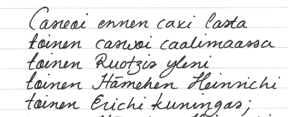(See the Results.) Primary Data-Set: Heinrichi The primary data-set is a result of an experiment performed by the organizers and 17 volunteers (see Credits). The original text is in old Finnish, and is known as Piispa Henrikin surmavirsi (‘The Death-Psalm of Bishop Henry’). Some of the copied variants are ‘missing’, i.e., not included in the given data-set. The copies were made by hand (pencil and paper). Note that the structure of the possible stemma is not necessarily limited to a bifurcating tree: more than two immediate descendants (children) and more than one immediate predecessor (parents) are possible. DownloadPlain text | Aligned text | Nexus format | ZIP | tar.gz New: The correct stemma and an evaluation script are available at the Causality workbench. Data-Set #2: Parzival (Validation Data) This is also an artificial data-set made by copying a text by hand. The correct solution will be made available during the challenge in order to enable self-assessment. This data-set will not affect the final results. '' If vaccilation dwell with the heart, the soul will see it. Shame and honour clash with the courage of a steadfast man is motley like a magpie. But such a man may yet make merry, for Heaven & Hell have equal part in him. ... '' The text is the beginning of the German poem Parzival by Wolfram von Eschenbach, translated to English by A.T. Hatto. The data was kindly provided to us by Matthew Spencer and Heather F. Windram. Download Plain text | Aligned table | Nexus format | ZIP | tar.gz Data-Set #3: Notre Besoin Another artificial data-set. The text is from Stig Dagerman’s, Notre besoin de consolation est impossible à rassasier, Paris: Actes Sud, 1952 (translated to French from Swedish by P. Bouquet), kindly provided to us by Caroline Macé. '' Je suis dépourvu de foi et ne puis donc être heureux, car un homme qui risque de craindre que sa vie ne soit errance absurde vers une mort certaine ne peut être heureux. ... '' DownloadPlain text | Aligned table | Nexus format | ZIP | tar.gz Data-Set #4: Legend of St. Henry This is a real data-set. The text is the Legend of St. Henry of Finland in Latin, written by the end of the 13th century at the latest. The surviving 52 versions are provided, some of which are severely damaged and fragmentary. For ease of use, the texts are aligned so that each line in the file contains one word, and empty lines are added so that the lines match across different files (e.g. the 50th line in each file contains the word pontificem unless that part of the manuscript is missing or damaged). The text is roughly 900 words long. DownloadPlain text | Aligned table | Nexus format | ZIP | tar.gz Procedures There are several data-sets included in the challenge. Some of them are real transcribed medieval manuscripts, some artificial (but hand-copied) ones. The data-sets are made available in (at least) two phases. Correct answers to some of the first phase data-sets will be announced before the final submission deadline in order to enable self-assessment by the participants. These data-sets will not affect the final results. Submissions are made in groups (of size one or more persons). Each group should submit at most two solutions. If more than two solutions are submitted, the last two before the deadline are accepted. A person can belong to at most two groups. (So a person can contribute to a maximum of four solutions.) Evaluation For the artificial data-sets, for which there is a known ‘ground-truth’ solution, the difference between the proposed and correct solutions is evaluation. The exact criterion is open for discussion among participants (and other interested parties). The current scoring function is based on distance orders among triplets (for details, see Example)  Go to Discussion. For the real data-sets, there is no known correct solution. Therefore, EBS¹ will be used: the ‘owner’ of the data-set will be asked to estimate whether the proposed solution is plausible and useful from his/her point of view. ¹ EBS: endorphin-based scoring Ranking Schemes There are two ranking schemes. Primary ranking is based on performance on the primary data-set (see Data Sets). Secondary ranking is based on all the other data sets except those for which the correct solution is annouced during the challenge, including both artificial and real data. For these other data sets, ‘thumbs-up’ marks will be awarded to the best submissions, and the total number of thumbs up determines the secondary ranking. The organizers reserve the right to alter the rules of the challenge at any point. Restrictions Anyone who has been in contact with some of the data-sets, or has otherwise obtained inside information about the correct solution should obviously not enter the challenge as regards the data-set(s) in question. However, participation is allowed as regards the other data-sets. The data-sets are provided only for the use in the challenge. Further use of the data requires an explicit permission by the organizers and the original providers of the data. Results Team*   Method** Data #1 Data #2 Data #3 Data #4*** Team Demokritos  n-gram clustering 64.4 % 79.3 % 66.4 % Rudi Cilibrasi CompLearn 52.7 % 81.5 % 70.6 % – Hierarchical clustering – 72.6 % 60.2 % – –  RHM06 76.0 % 79.9 % 76.9 % – –  PAUP: Parsimony 74.4 % 77.8 % 74.5 % – –  PAUP: Neighbour Joining 64.4 % 81.5 % 76.2 % – –  PAUP: Least Squares 64.2 % 81.5 % 70.2 % – –  SplitsTree: NeighborNet 59.1 % 77.8 % 70.2 % – –  SplitsTree: SplitDecomposition 53.1 % 74.5 % 73.1 % – –  SplitsTree: ParsimonySplits 56.8 % 83.7 % 71.6 % – *) The entries below the horizontal line are added for comparison purposes by the organizers, and, therefore, not included in the competition. **) RHM06 = (Roos, Heikkilä, Myllymäki, “A Compression-Based Method for Stemmatic Analysis”, ECAI-06). PAUP = PAUP* version 4.0b10 for Unix. Heuristic search. SplitsTree = SplitsTree4 version 4.10, build 2, May 2008. ***) Data #4 is ‘real’ and no correct solution is known. The winner in the primary ranking (Data #1) is Team Demokritos (click on the team title in the table for more information). The secondary ranking is based on Data #3 and Data #4 for which the winner is Rudi Cilibrasi who’s submission was the best for Data #3. Neither submission was “plausible and useful” for Data #4 (as judged by a domain expert, hence no points for anyone).

The objective of the Challenge is to design a statistical machine learning algorithm that discovers which morphemes (smallest individually meaningful units of language) words consist of. Ideally, these are basic vocabulary units suitable for different tasks, such as text understanding, machine translation, information retrieval, and statistical language modeling.

The scientific goals are:

• To learn of the phenomena underlying word construction in natural languages
• To discover approaches suitable for a wide range of languages
• To advance machine learning methodology

Morpho Challenge 2007 is a follow-up to our previous Morpho Challenge 2005 (Unsupervised Segmentation of Words into Morphemes). The task of Morpho Challenge 2007 is more general in that we are not necessarily looking for an explicit segmentation of words this time, but a morpheme analysis of the word forms in the data. (For instance, the English words “boot, boots, foot, feet” might obtain the analyses “boot, boot + plural, foot, foot + plural”, respectively.)

Participation in the previous challenge is by no means a prerequisite for participation in Morpho Challenge 2007. Everyone is welcome and we hope to attract many participating teams. The results will be presented in a workshop arranged in conjunction with CLEF 2007 (Cross-Language Evaluation Forum). Please read the rules and see the schedule. The datasets are available for download. Submit your analyses (result files) by sending them by email to the organizers, or by indicating a location where the organizers can download your files. Remember also to describe your algorithm in an extended abstract. Please read the formatting instructions in rules.

The result tables from the latest evaluation runs are now in the Results page.

We are looking forward to an interesting competition!

Mikko Kurimo, Mathias Creutz and Matti Varjokallio
Adaptive Informatics Research Centre, Helsinki University of Technology
The organizers

Program committee

Levent Arslan, Boğaziçi University
Eric Atwell, University of Leeds
Samy Bengio, Google
Tolga Cilogu, Middle-East Technical University
Kadri Hacioglu, Colorado University
Colin de la Higuera, Jean Monnet University, Saint-Etienne
Chun Yu Kit, City University of Hong Kong
Dietrich Klakow, Saarland University
James Martin, University of Colorado at Boulder
Jan Nouza,Technical University of Liberec
Erkki Oja, Helsinki University of Technology
Murat Saraçlar, Boğaziçi University
Richard Sproat, University of Illinois, Urbana-Champaign
Richard Wicentowski, Swarthmore College

Rules

Acceptance

The organizers retain all rights to the Challenge data, which is given to the participants for use in this challenge only. The organizers may use the data submitted to the Challenge freely, without restrictions.

Eligibility

Anyone is allowed to participate. A participant may be either a single person or a group. A single person can participate in at most two groups. A participant is allowed to submit at most three different solutions, where each solution corresponds to a particular morpheme analysis method. Each of these methods may naturally be applied to each of the test languages. If a participant submits more than three solutions, the organizers decide which of the three will be accepted.

Test languages

Data sets are provided for four languages: English, Finnish, German and Turkish. Participants are encouraged to apply their algorithm to all of these test languages, but are free to leave some languages out, if they wish to do so.

(New languages may be added, if interested co-organizers, suitable data and evaluation analyses become available in time.)

Task

The task is the unsupervised morpheme analysis of every word form contained in a word list supplied by the organizers for each test language.

The participants will be pointed to corpora in which the words occur, so that the algorithms may utilize information about word context.

Solutions, in which a large number of parameters must be “tweaked” separately for each test language, are of little interest. This challenge aims at the unsupervised (or very minimally supervised) morpheme analysis of words. The abstracts submitted by the participants must contain clear descriptions of which steps of supervision or parameter optimization are involved in the algorithms.

Competitions

The segmentations will be evaluated in two complementary ways:

• Competition 1: The proposed morpheme analyses will be compared to a linguistic “gold standard”.
• Competition 2: Information retrieval (IR) experiments will be performed, where the words in the documents and queries will be replaced by their proposed morpheme representations. The search will then be based on morphemes instead of words.

Competition 1 will include all four test languages. Winners will be selected separately for each language. As a performance measure, the F-measure of accuracy of suggested morpheme analyses is utilized. Should two solutions produce the same F-measure, the one with higher precision will win.

Competition 2 will include three of the test languages. The organizers will perform the IR experiments based on the morpheme analyses submitted by the participants.

Workshop and publication

All good results will be acknowledged with fame and glory. Presentations for the challenge workshop will be selected by the program committee based on the results and an extended abstract of at most 6 pages.

Extended abtracts

For the extended abstract you can use the two-column ACL/COLING format (figures and tables may still span the whole width of a page). Detailed formatting instructions can be found here: PDF or PS. You can use the following files: Latex style file, Latex bibliography file, and a template Latex document. The maximum length of your paper is 6 pages (including references and figures). Email your extended abstract to the organizers by May 31.

Camera-ready submission

The final camera-ready submissions use a different format than the papers submitted for review. We are sorry about the inconvenience of your having to reformat your documents. For your final paper submission (due August 15th), please use the single-column CLEF 2007 Notebook Proceedings format. Here are a sample PDF file and a template Latex document. Detailed formatting instructions can be requested from the Morpho Challenge Organizers. The maximum length of your paper is 10 pages (including references and figures), but you can ask for a couple of extra pages if you think it improves the paper. Email your final paper to the organizers.

Arbitration

In the case of disagreement the organizers will decide the final interpretation of the rules.

Datasets

There are a number of data files involved in this challenge. Each type of file is available for each language.

Word list (input)

First and foremost, there is a list of word forms. The words have been extracted from a text corpus, and each word in the list is preceded by its frequency in the corpus used.

For instance, a subset of the supplied English word list looks like this:

...
1 barefoot's
2 barefooted
6699 feet
653 flies
2939 flying
1782 foot
64 footprints
...

Result file (output, i.e., what to submit)

The participants’ task is to return a list containing exactly the same words as in the input, with morpheme analyses provided for each word. The list returned shall not contain the word frequency information.

A submission for the above English words may look like this:

...
barefoot's      BARE FOOT +GEN
barefooted      BARE FOOT +PAST
feet            FOOT +PL
flies           FLY_N +PL, FLY_V +3SG
flying          FLY_V +PCP1
foot            FOOT
footprints      FOOT PRINT +PL
...

There are a number of things to note about the result file: Each line of the file contains a word (e.g., “feet”) separated from its analysis (e.g., “FOOT +PL”) by one TAB character. The word needs to look exactly as it does in the input; no capitalization or change of character encoding is allowed. The analysis contains morpheme labels separated using space. The order in which the labels appear does not matter; e.g., “FOOT +PL” is equivalent to “+PL FOOT”. The labels are arbitrary: e.g., instead of using “FOOT” you might use “morpheme784” and instead of “+PL” you might use “morpheme2”. However, we strongly recommend you to use intuitive labels, when possible, since they make it easier for anyone to get an idea of the quality of the result by looking at it.

If a word has several interpretations, all interpretations should be supplied: e.g., the word “flies” may be the plural form of the noun “fly” (insect) or the third person singular present tense form of the verb “to fly”. The alternative analyses must be separated using a comma, as in: “FLY_N +PL, FLY_V +3SG”. The existence of alternative analyses makes the task challenging, and we leave it to the participants to decide how much effort they will put into this aspect of the task. In English, for instance, in order to get a perfect score, it would be necessary to distinguish the different functions of the ending “-s” (plural or person ending) as well as the different parts-of-speech of the stem “fly” (noun or verb). As the results will be evaluated against reference analyses (our so-called gold standard), it is worth reading about the guiding principles used when constructing the gold standard.

As far as we understand, you can use any characters in your morpheme labels except whitespace and comma (,). However, we cannot guarantee that the evaluation scripts will work properly, if your labels contain some “strange” characters.

Text corpus

The word list (input data) has been constructed by collecting word forms occurring in a text corpus. The text corpora have been obtained from the Wortschatz collection at the University of Leipzig (Germany). We used the plain text files (sentences.txt for each language); the corpus sizes are 3 million sentences for English, Finnish and German, and 1 million sentences for Turkish. For English, Finnish and Turkish we use preliminary corpora, which have not yet been released publicly at the Wortschatz site. The corpora have been preprocessed for the Morpho Challenge (tokenized, lower-cased, some conversion of character encodings).

If the participants like to do so, they can use the corpora in order to get information about the context in which the different words occur.

We are most grateful to the University of Leipzig for making these resources available to the Challenge, and in particular we thank Stefan Bordag for his kind assistance.

Gold standard morpheme analyses

The desired “correct” analyses for a random sample of circa 500 words are supplied for each language. These samples can be used for visual inspection and as a development test set (in order to get a rough estimate of the performance of the participants’ morpheme-analyzing algorithm).

The format of the gold standard file is exactly the same as that of the result file to be submitted. That is, each line contains a word and its analysis. The word is separated from the analysis by a TAB character. Morpheme labels in the analysis are separated from each other by a space character. For some words there are multiple correct analyses. These alternative analyses are separated by a comma (,). Examples:

The English and German gold standards are based on the CELEX data base. The Finnish gold standard is based on the two-level morphology analyzer FINTWOL from Lingsoft, Inc. The Turkish gold-standard analyses have been obtained from a morphological parser developed at Boğaziçi University; it is based on Oflazer’s finite-state machines, with a number of changes. We are indebted to Ebru Arısoy for making the Turkish gold standard available to us.

The morphological analyses are morpheme analyses. This means that only grammatical categories that are realized as morphemes are included. For instance, for none of the languages will you find a singular morpheme for nouns or a present-tense morpheme for verbs, because these grammatical categories do not alter or add anything to the word form, in contrast to, e.g., the plural form of a noun (house vs. house+s), or the past tense of verbs (help vs. help+ed, come vs. came).

The morpheme labels that correspond to inflectional (and sometimes also derivational) affixes have been marked with an initial plus sign (e.g., +PL, +PAST). This is due to a feature of the evaluation script: in addition to the overall performance statistics, evaluation measures are also computed separately for the labels starting with a plus sign and those without an initial plus sign. It is thus possible to make an approximate assessment of how accurately affixes are analyzed vs. non-affixes (mostly stems). If you use the same naming convention when labeling the morphemes proposed by your algorithm, this kind of statistics will be available for your output (see the evaluation page for more information).

The morpheme labels that have not been marked as affixes (no initial plus sign) are typically stems. These labels consist of an intuitive string, usually followed by an underscore character (_) and a part-of-speech tag, e.g., “baby_N”, “sit_V”. In many cases, especially in English, the same morpheme can function as different parts-of-speech; e.g., the English word “force” can be a noun or a verb. In the majority of these cases, however, if there is only a difference in syntax (and not in meaning), the morpheme has been labeled as either a noun or a verb, throughout. For instance, the “original” part-of-speech of “force” is a noun, and consequently both noun and verb inflections of “force” contain the morpheme “force_N”:

Thus, there is not really a need for your algorithm to distinguish between different meanings or syntactic roles of the discovered stem morphemes. However, in some rare cases, if the meanings of the different parts-of-speech do differ clearly, there are two variants, e.g., “train_N” (vehicle), “train_V” (to teach), “fly_N” (insect), “fly_V” (to move through the air). But again, if there are ambiguous meanings within the same part-of-speech, these are not marked in any way, e.g., “fan_N” (device for producing a current of air) vs. “fan_N” (admirer). This notation is a consequence of using CELEX and FINTWOL as the sources for our gold standards. We could have removed the part-of-speech tags, but we decided to leave them there, since they carry useful information without significantly making the task more difficult. There are no part-of-speech tags in the Turkish gold standard.

Random word pairs file

If you want to carry out a small-scale evaluation yourself using the gold standard sample, you need to download a randomly generated so-called word pairs file for each language to be tested. Read more about this on the evaluation page.

Character encoding

In the source data used for the different languages, there is variation in how accurately certain distinctions are made when letters are rendered. This makes it hard to apply a unified character encoding scheme for all the languages (such as UTF-8). Thus, the following encodings have been used, in which all letters are encoded as one-byte (8-bit) characters:

English

Standard text. All words are lower-cased, also proper names.

Finnish

ISO Latin 1 (ISO 8859-1). The Scandinavian special letters å, ä, ö (as well as other letters occuring in loan words, e.g., ü, é, à) are rendered as one-byte characters. All words are lower-cased, also proper names.

German

Standard text. All words are lower-cased, also all nouns. The German umlaut letters are rendered as the corresponding non-umlaut letter followed by “e”, e.g., “laender” (Länder), “koennte” (könnte), “fuer” (für). Double-s is rendered as “ss”, e.g., “strasse” (Straße). This coarse encoding is due to the fact that CELEX, the source for the morphological gold standard, utilizes this scheme. Note, however, that in the data you may see special letters encoded using ISO Latin 1 in some loan words, e.g., “société”, “l’unità” (these words are not included in CELEX and their analyses will not be evaluated).

Turkish

Standard text. All words are lower-cased. The letters specific to the Turkish language are replaced by capital letters of the standard Latin alphabet, e.g., “açıkgörüşlülüğünü” is spelled “aCIkgOrUSlUlUGUnU”.

Download

Instead of downloading each file separately, you can download the whole package, either as a tar/gzip file: morphochal07data.tgz (530 MB; unpack using “tar xzf“) or as a zip file: morphochal07data.zip (540 MB).

Competition 1

In Competition 1, for each language, the morpheme analyses proposed by the participants’ algorithm will be compared against a linguistic gold standard. Samples of the gold standards used are available for download on the datasets page.

Since the task at hand involves unsupervised learning, it cannot be expected that the algorithm comes up with morpheme labels that exactly correspond to the ones designed by linguists. That is, no direct comparison will take place between labels as such (the labels in the proposed analyses vs. labels in the gold standard). What can be expected, however, is that two word forms that contain the same morpheme according to the participants’ algorithm also have a morpheme in common according to the gold standard. For instance, in the English gold standard, the words “foot” and “feet” both contain the morpheme “foot_N”. It is thus desirable that also the participants’ algorithm discovers a morpheme that occurs in both these word forms (be it called “FOOT”, “morpheme784”, “foot” or something else).

In practice, the evaluation will take place by sampling a large number of word pairs, such that both words in the pair have at least one morpheme in common. As the evaluation measure, we will use F-measure, which is the harmonic mean of Precision and Recall:

F-measure = 1/(1/Precision + 1/Recall).

Precision is here calculated as follows: A number of word forms will be randomly sampled from the result file provided by the participants; for each morpheme in these words, another word containing the same morpheme will be chosen from the result file by random (if such a word exists). We thus obtain a number of word pairs such that in each pair at least one morpheme is shared between the words in the pair. These pairs will be compared to the gold standard; a point is given for each word pair that really has a morpheme in common according to the gold standard. The total number of points is then divided by the total number of word pairs.

For instance, assume that the proposed analysis of the English word “abyss” is: “abys +s”. Two word pairs are formed: Say that “abyss” happens to share the morpheme “abys” with the word “abysses”; we thus obtain the word pair “abyss – abysses”. Also assume that “abyss” shares the morpheme “+s” with the word “mountains”; this produces the pair “abyss – mountains”. Now, according to the gold standard the correct analyses of these words are: “abyss_N”, “abyss_N +PL”, “mountain_N +PL”, respectively. The pair “abyss – abysses” is correct (common morpheme: “abyss_N”), but the pair “abyss – mountain” is incorrect (no morpheme in common). Precision here is thus 1/2 = 50%.

Recall is calculated analogously to recall: A number of word forms are randomly sampled from the gold standard file; for each morpheme in these words, another word containing the same morpheme will be chosen from the gold standard by random (if such a word exists). The word pairs are then compared to the analyses provided by the participants; a point is given for each sampled word pair that has a morpheme in common also in the analyses proposed by the participants’ algorithm. The total number of points is then divided by the total number of word pairs.

For words that have several alternative analyses, as well as for word pairs that have more than one morpheme in common, some normalization of the points is carried out in order not to give these words considerably more weight in the evaluation than “less complex” words. We will spare the participants from the gory details. (The passionately interested reader may have a look at the source code of the evaluation script.)

Evaluation of a sample (development test set)

You can evaluate your morphological analyses against the available gold standards (separately for each test language). The program to use for this is the Perl script: eval_morphemes.pl. The evaluation program is invoked as follows:

eval_morphemes.pl [-trace] wordpairsfile_goldstd wordpairsfile_result goldstdfile resultfile

Four files are given as arguments to eval_morphemes.pl:

1. wordpairsfile_goldstd: this is the “random word pairs file” available for download on the datasets page. This file is needed in the calculation of an estimate of the recall of the proposed morpheme analyses.
2. wordpairsfile_result: this file has to be generated using another program (see below). It is needed in the calculation of a rough estimate of the precision of the proposed morpheme analyses.
3. goldstdfile:this is the sample of the gold standard available for download on the datasets page. This file contains the correct morpheme analyses for circa 500 words.
4. resultfile: this is the result file that your algorithm produces, i.e., a list of words and their proposed morpheme analyses.

The -trace argument is optional and produces output for every evaluated word separately. Regardless of the status of the trace argument, the evaluation program produces output of the following kind:

PART0. Precision: 69.00% (96/139); non-affixes: 81.55% (51/63); affixes: 58.73% (45/76)
PART0. Recall:    25.59% (142/556); non-affixes: 49.78% (105/211); affixes: 10.78% (37/345)
PART0. F-measure: 37.33%; non-affixes: 61.82%; affixes: 18.22%
#
TOTAL. Precision: 69.00%; non-affixes: 81.55%; affixes: 58.73%
TOTAL. Recall:    25.59%; non-affixes: 49.78%; affixes: 10.78%
TOTAL. F-measure: 37.33%; non-affixes: 61.82%; affixes: 18.22%

Note that results are displayed for partition 0 (PART0) and for the entire data (TOTAL). The total scores are here the same as the scores of PART0, since there is only one partition. It is, however, possible to split the data into several partitions and compute results for each partition separately. The overall scores are then calculated as the mean over the partitions. Splitting into partitions is a feature reserved for the final evaluation, when we will assess the statistical significance of the differences between the participants’ algorithms.

The figures that count in the final evaluation are the first precision, recall, and F-measure values on the TOTAL lines. These values pertain to all morphemes, but there are also separate statistics for morphemes classified as non-affixes vs. affixes. What counts as an affix is a morpheme with a label starting with a plus sign, e.g., “+PL”, “+PAST”. This naming convention is applied in the gold standard, which means that you do not have to do anything in order to get the non-affixes/affixes statistics right as far as recall is concerned. However, if you want the same kind of information also for precision, your algorithm must have a means of discovering which morphemes are likely affixes and tag these morphemes with an initial plus sign. Note that it is fully up to you whether you do this or not; it will not affect your position in the competition in any way.

Sampling word pairs for the calculation of an estimate of the precision

In order to get an estimate of the precision of the algorithm, you need to provide the evaluation script eval_morphemes.pl with a file containing word pairs sampled from your result file. Unfortunately, the estimate is likely to be fairly rough. The reason for this is that you do not have the entire gold standard at your disposal. Thus, if you sample pairs of words that are not included in the 500-word gold standard that you can access, it is impossible to know whether the proposed morphemes are correct or not. What you can do, however, is to make sure that each word that goes into a word pair actually does occur in the 500-word gold standard sample. The problem here is that your algorithm might not propose that many common morphemes for the words within this limited set, and thus the estimate will be based on rather few observations.

Anyway, this is how to do it: First, make a list of relevant words, that is, words that are present in the gold standard sample available:

cut -f1 goldstdfile > relevantwordsfile

Then sample word pairs for 100 words selected by random from your results file:

sample_word_pairs.pl -refwords relevantwordsfile < resultfile > wordpairsfile_result

The necessary Perl program is sample_word_pairs.pl. The output file wordpairsfile_result is used as input to eval_morphemes.pl (see above).

Competition 2

Competition 2 does not require any extra effort by the participants. The organizers will use the analyses provided by the participants in information retrieval experiments. Data from CLEF will be used. It is possible that no evaluation data for Turkish will be available for Competition 2.

The words in the queries and documents will be replaced by the corresponding morpheme analyses provided by the participants. We will perform the evaluation using a state-of-the-art retrieval method (the latest version of the freely available LEMUR toolkit, and the evaluation criterion will be Uninterpolated Average Precision. The segmentation with the highest Average Precision will win. The winner is selected separately for each language and these 4 different indexing runs in each language:

1. All morphemes from the training data are used as index terms, Tfidf (BM25) weighting for all
2. Additional morphemes from the IR data used, too, Tfidf (BM25) weighting for all
3. All morphemes from the training data are used as index terms, Okapi (BM25) weighting for all except the most common ones (stoplist)
4. Additional morphemes from the IR data used, too, Okapi (BM25) weighting for all except the most common ones (stoplist)

Results

This page contains only the result tables from the latest evaluation runs. The full evaluation report was published at the Workshop.

Competition 1

The segmentation with the highest F-measure is the best. The winner is selected separately for each language.
Download the report on the final results from here.

Finnish
Turkish
German
English

Competition 2

In Competition 2, the organizers applied the analyses provided by the participants in information retrieval experiments. The words in the queries and source documents were replaced by the corresponding morpheme analyses provided by the participants, and the search was then based on morphemes instead of words. The evaluation was perfomed using a state-of-the-art retrieval method (the latest version of the freely available LEMUR toolkit. The evaluation criterion was Uninterpolated Average Precision There were several different categories in Competition 2 and the winner with the highest Average Precision was selected separately for each language and each category:

1. All morpheme analysis from the training data are used as index terms “withoutnew” vs. additionally using also the morpheme analysis for new words that existed in the IR data but not in the training data “withnew”.
2. Tfidf (BM25) term weighting was utilized for all index terms without any stoplists vs. Okapi (BM25) term weighting for all index terms excluding an automatic stoplist consisting of 75,000 (Finnish) or 150,000 (German and English) most common terms. The stoplist was used with the Okapi weighting, because it did not perform well with the indexes that had many very common terms.

Download the report on the final results from here.

Finnish
German
English

Proceedings

The proceedings are available in CLEF working notes.
The manuscripts and abstracts can be downloaded from here.

Reference methods

To study how the different morpheme analysis performed in the IR tasks, we attempted the same tasks with different reference methods. This also revealed us whether the unsupervised morpheme analysis (or even a supervised one) could really be useful in the IR tasks compared to simple word based indexing.

1. Morfessor Categories-Map: The same Morfessor Categories-Map as described in Competition 1 was used for the unsupervised morpheme analysis. The stem vs. suffix tags were kept, but did not receive any special treatment in the indexing as we wanted to keep the IR evaluation as unsupervised as possible.
2. Morfessor Baseline: All the words were simply split into smaller pieces without any morpheme analysis. This means that the obtained subword units were directly used as index terms as such. This was performed using the Morfessor Baseline algorithm as in Morpho Challenge 2005. We expected that this would not be optimal for IR, but because the unsupervised morpheme analysis is such a difficult task, this simple method would probably do quite well.
3. dummy: No words were split nor any morpheme analysis provided. This means the all were directly used as index terms as such without any stemming or tags. We expected that although the morpheme analysis should provide helpful information for IR, all the submissions would not probably be able to beat this brute force baseline. However, if some morpheme analysis method would consistently beat this baseline in all languages and task, it would mean that the method were probably useful in a language and task independent way.
4. grammatical: The words were analysed using the gold standard in each language that were utilised as the “ground truth” in the Competition 1. Besides the stems and suffixes, the gold standard analyses typically consist of all kinds of grammatical tags which we decided to simply include as index terms, as well. For many words the gold standard analyses included several alternative interpretations that were all included in the indexing. However, we decided to also try the method adopted in the morpheme segmentation for Morpho Challenge 2005 that only the first interpretation of each word is applied. This was here called “grammatical first” whereas the default was called “grammatical all”. Because our gold standards are quite small, 60k (English) – 600k (Finnish), compared to the amount of words that the unsupervised methods can analyse, we did not expect “grammatical” to perform particularly well, even though it would probably capture some useful indexing features to beat the “dummy”, at least.
5. Porter: No real morpheme analysis was performed, but the words were stemmed by the Porter stemming, an option provided by the Lemur toolkit. Because this is quite standard procedure in IR, especially for English text material, we expected this to provide the best results, at least for English. For the other languges the default Porter stemming was not likely to perform very well.
6. Tepper: A hybrid method developed by Michael Tepper was utilized to improve the morpheme analysis reference obtained by our Morfessor Categories-MAP. Based on the obtained performance in Competition 1, we expected that this could provide some interesting results here, as well.

What is it about?

The goal of this challenge is to attract the attention of the Machine Learning community towards the problem where the input distributions, p(x), are different for test and training inputs. A number of regression and classification tasks are proposed, where the test inputs follow a different distribution than the training inputs. Training data (input-output pairs) are given, and the contestants are asked to predict the outputs associated to a set of validation and test inputs. Probabilistic predictions are strongly encouraged, though non-probabilitic “point” predictions are also accepted. The performance of the competing algorithms will be evaluated both with traditional losses that only take into account “point predictions” and with losses that evaluate the quality of the probabilistic predictions.

Results

We are proud to announce the two challenge winners:

• Gavin C. Cawley
• Debajyoti Ray

Congratulations!

For a summary of the results, click on the “Results” tab.

How do I participate?

The first phase of the challenge is over, the results are summarized in the “Results” tab.
It is still possible to submit predictions and get them evaluated by the challenge server!

• Download the datasets (“Datasets” in left frame)
• Look at the evaluation criteria (“Evaluation”)
• Format your predictions on the test inputs as required (“Instructions”)
• Submit your results (“Submission”)
• See how well you do compared to others (“Results”)

Where can we discuss the results?

There will be a workshop on this topic at the NIPS*2006 conference. The results of the competition will be announced there as well. More information about the workshop can be found here.

Background

Many machine learning algorithms assume that the training and the test data are drawn from the same distribution. Indeed many of the proofs of statistical consistency, etc., rely on this assumption. However, in practice we are very often faced with the situation where the training and the test data both follow the same conditional distribution, p(y|x), but the input distributions, p(x), differ. For example, principles of experimental design dictate that training data is acquired in a specific manner that bears little resemblance to the way the test inputs may later be generated.

The open question is what to do when training and test inputs have different distributions. In statistics the inputs are often treated as ancillary variables. Therefore even when the test inputs come from a different distribution than the training, a statistician would continue doing “business as usual”. Since the conditional distribution p(y|x) is the only one being modelled, the input distribution is simply irrelevant. In contrast, in machine learning the different test input distribution is often explicitly taken into account. An example is semi-supervised learning, where the unlabeled inputs can be used for learning. These unlabeled inputs can of course be the test. Additionally, it has recently proposed to re-weight the training examples that fall in areas of high test input density for learning (Sugiyama and Mueller, 2005). Transductive learning, which concentrates the modelling at the test inputs, and the problem of unbalanced class labels in classification, particularly where this imbalance is different in the training and in the test sets, are both also very intimately to the problem of different input distributions.

It does not seem to be completely clear, whether the benefits of explicitly accounting for the difference between training and test input distributions outweigh the potential dangers. By focusing more on the training examples in areas of high test input density, one is effectively throwing away training data. Semi-supervised learning on the other hand is very dependent on certain prior assumptions being true, such as the cluster assumption for classification.

The aim of this challenge is to try and shed light on the kind of situations where explicitly addressing the difference in the input distributions is beneficial, and on what the most sensible ways of doing this are. For this purpose, we bring the theoretical questions to the empirical battleground. We propose a number of regression and classification datasets, where the test and training inputs have different distributions.

Deadline and Number of Submissions

• The deadline for final submissions is November 24, 2006.
• Please observe limit of at most 5 submissions per day on a given dataset.

Instructions for Submission

• One submission is associated to one dataset, and consists of a file compressed with “zip”. The name of the compressed file is irrelevant, only its extension is important.
• Zip programs are available for most operating systems, including Microsoft Windows, Linux and Mac OS. If, however, you do not have a zip program installed on your system yet, you can find download links on the tools page.
• The compressed file should contain one ascii file for each split of the data (training, validation and test). The names are important, and must follow the following convention:
  • datasetname_train_predict.txt
  • datasetname_val_predict.txt
  • datasetname_test_predict.txt (only after November 10)
• Example: to submit your results for the “barley” dataset do
  > zip results.zip barley_train_targets.txt barley_val_targets.txt barley_test_targets.txt

  Validation phase and test phase

  Until November 10, the challenge will be in its validation phase: only the validation inputs will be available, and therefore only the validation predictions will be evaluated. On November 10, the test inputs will be released, as well as the validation targets, and the test phase will start, which will last until the deadline for submissions of November 24. During the validation phase, the losses of the submissions will be immediately displayed in the results page. During the test phase however, no results will be shown. This is to avoid the temptation of fine tuning the algorithms by using the feedback provided by the test score. The final ranking will be built according to the test scores. During the validation phase, submissions will be ranked according to the validation score, to allow participants to get an idea of how their method does.

Format of the ASCII files

• Both for regression and classification, the ASCII files should contain one prediction per row.
• The predictions must be made in the same order as the inputs appear in the data files. For example, the file “barley_val_predict.txt” should contain 300 rows, as many as validation examples.
• Exponential notation is accepted, in the form 6.7125064e-01.
  (Matlab’s default when saving to ASCII files)

Classification

For classification, one prediction is equal to , which is a number in corresponding to the estimated (posterior) probability of input of belonging to class ““.
To produce non-probabilistic predictions in classification, just return “hard” probabilities of belonging to class “+1”, equal to either “1” or to “0”.

Regression

For regression, one prediction is a set of numbers that describe some aspects of the predictive distribution .

• by providing the mean and variance of a Gaussian predictive distribution:To declare that the mean and variance of a Gaussian predictive distribution are specified, the corresponding row of the ASCII file must start with a “” and then contain the mean and the variance. For example, if the estimated has mean and variance , the j-th line of the ASCII file should be:To produce non-probabilistic predictions in regression, produce Gaussian predictions with the mean equal to your “point prediction”, and the variance equal to 0.
• by providing a set of quantiles that describe the predictive distribution:To use quantiles to describe the predictive distribution, the corresponding row of the ASCII file should start with a ““, and be followed by a number of pairs of probabilities and associated quantiles. To describe the estimated predictive distribution with quantiles, the j-th row of the ASCII file should look like:where for all the ‘s are cumulative probabilities that obey , and the participant is free to choose their number (although 200 is the maximum) () and their values.For a given , the corresponding quantile is computed from the predictive (of the true target distribution) as:

  (1)

It is possible to use both ways of describing prediction distributions for different predictions in the same ASCII file.

Datasets for Classification

Name	Size	Features	Training Examples	Validation Examples	Test Examples	Link
Wheat	37 KB	5	400	50	1000
Barley	37 KB	5	400	50	1000
Schnitzel	5 KB	3	280	40	185

Format of the datasets

• Each dataset is contained in a folder compressed with zip
• Each dataset comprises 3 ascii files named
  • [dataset_name]_train_inputs.txt
  • [dataset_name]_train_targets.txt
  • [dataset_name]_val_inputs.txt
• Rows correspond to examples, columns to dimensions

NEW! (13.11.06) The final version of the datasets has been released. You need to download the whole data again

On November 10, a new version of the datasets will be released, which will include the two following files in addition to the above:

• [dataset_name]_val_targets.txt (available after November 10)
• [dataset_name]_test_inputs.txt (available after November 10)

to obtain them, you will have to download the datasets again from this page.

Script for computing losses

You can download a python script called ‘evaluate.py’ for computing the different losses [here]

Usage:
>> python evaluate.py your_prediction_file true_targets_file loss_type

where loss_type is a number from 1 to 4 with the meaning:

• Regression: 1 = NLPD, 2 = MSE
• Classification: 3 = NLP, 4 = 01L

The files with your predictions and with the true targets should be formatted in the usual way for this challenge.

Measures for Evaluation of Performance

We plan to use losses that both allow to evaluate the quality of the predictive distributions, and standard losses that evaluate deterministic predictions.

Suppose in all cases that there are test (or validation) input/output pairs:

Ranking

For each dataset, the methods of the participants will be ranked from best to worst.

• The test performance will not be evaluated until after the deadline for submission (November 24, 2006).
• In the meantime, the methods will be ranked according to their NLP (see below) performance on the validation set.
• One week before the deadline for submissions the targets of the validation set will be made public for the use of the participants.

Losses for Classification

In classification, the true labels can only take values “” or ““. We use the following two losses:

• [NLP] Average negative log estimated predictive probability of the true labels:

  (1)

  Notice that this loss penalizes both over and under-confident predictions. Over-confident predictions can be infinitely penalized, so we discourage contestants to submit predictive probabilities equal to 1. Zero is the minimum value of this loss, that one could achieve if one predicted correctly with 100% confidence. If one predicts otherwise, the worse one predicts, the larger the loss. This loss is also referred to as “negative cross-entropy loss”.

• [01L] Average classification error (0/1 loss):

  (2)

  where is the indicator function.
  This is the classic 0/1 loss, obtained by thresholding the predictive probabilities about 0.5. Its minimum value is 0, obtained when no test (or validation) examples where missclassified; it is otherwise equal to the fraction of missclassified examples relative to the total number of examples.

Losses for Regression

In regression, the true labels are real valued numbers. We use the following two losses:

• [NLPD] Average negative log estimated predictive density of the true targets:

  (7)

  This measure penalizes over-confident predictions as well as under-confident ones.

• [MSE] Mean squared error (normalized):

  (8)

  where is the mean of the estimated predictive distribution . We normalize the loss by the empirical variance of the training data, . This classical loss takes only into account a point prediction that minimizes squared errors. Given the predictive distribution, this optimal point prediction is its mean.

How are the losses obtained from quantiles?

• If the participant describes a predictive distribution by a Gaussian (mean and variance), the losses for regression are straightforward to compute.
• If the participant describes a predictive distribution by a number of quantiles, we approximate the density at the true target, and we obtain an approximation to the predictive mean. Please find the details in the following document [pdf]

Summary of the Results

We are proud to announce the two challenge winners:

• Gavin C. Cawley
• Debajyoti Ray

Congratulations!

In the following, we list the best 3 submissions for each data set, based on the submissions that were received until November 24, 2006. For updated results that also include submissions after November 24, click here (classification) or or here (regression).

Udon (Regression)

“Udon” are samples from a noisy sine function. The data set is inspired by the toy data set in Sugiyama and Mueller (2006), where the function suddenly changes from sine to linear right at the border between training and test data. Here, this slightly surprising change does not occur.

A number of people only submitted results for validation data (Jukka Kohonen, Cyril Goutte).

Gavin Cawley writes about his winning submission: “simple sinusoidal model with parameters representing the amplitude, frequency and offset. Fitted using leave-one-out cross- validation. The variance estimator was augmented by a component representing the variance of the leave-one-out estimates, to give a slightly heteroscedastic variance (although this didn’t make much difference).”

Maki (Regression)

Maki represents a depth from stereo experiment. Actually, this is an ordinal regression dataset – still, we evaluate it as standard regression. The difficulty here is that training data were chosen only from a number of planes, wheres test data are chosen from all planes.

Gavin Cawley writes about his winning submission: “They are all kernel ridge regression models, with the regularisation and kernel parameters set so as to minimise the leave-one-out error. #1: linear, #2: quadratic, #3: cubic, #4: rbf, #5: rbf with feature scaling”

Schnitzel (Classification)

Here comes the real world! The Schnitzel data set stems from a Brain-Computer-Interface (BCI) experiment (“Schnitzel” is the nickname of the subject in this experiment).

Training data stem from the BCI training session, validation and test data were taken from the BCI feedback session. The big challenge here is that training and test exhibit neurophysiological differences. Thus, this data set is actually an “outlier”, in that not only the input distribution of training and test is different, but also the conditional distribution changes.

So, in a way, this is Mission Impossible. The baseline achievable here (classifier on training data only) is around 40% error rate. With a classifier that does a sequential update when test targets become available, it is possible to reach around 32% error rate.

Gavin Cawley writes about his submission: “performed a PCA (on all three sets) and discarded the first principal component (as the training data has discriminative informaation in this direction that was not compatible with the test and validation sets having many positive patterns). I think submissions 1 and 2 are just kernel logistic regression models. A logistic regression model was used, with a simple form of Baysian transduction on submission #4.”

Barley (Classification)

Barley is the 5-dimensional version of the following data set: (blue and black are the training data, red is the test data)

Gavin Cawley writes about his submission: “They are all kernel ridge regression models, with the regularisation and kernel parameters set so as to minimise the leave-one-out error, the kernels used are in the following order: #1 linear, #2 quadratic, #3 cubic, #4 rbf, #5 rbf with feature scaling. #6is logistic regresion with Bayesian transduction, but it needs work, it was a bit of a hack!”

Wheat (Classification)

Wheat is the 5-dimensional version of the following data set: (blue and black are the training data, red is the test data)

Gavin Cawley writes about his winning submission: ” They are all kernel ridge regression models, with the regularisation and kernel parameters set so as to minimise the leave-one-out error, the kernels used are in the following order: #1 linear, #2 quadratic, #3 cubic, #4 rbf, #5 rbf with feature scaling. #6is logistic regresion with Bayesian transduction, but it needs work, it was a bit of a hack!”

RTE-3 followed the same basic structure of the previous campaigns, in order to facilitate the participation of newcomers and to allow “veterans” to assess the improvements of their systems in a comparable test exercise. Nevertheless, some innovations were introduced, on the one hand to make the challenge more stimulating and, on the other, to encourage collaboration between system developers. In particular, a limited number of longer texts, i.e. up to a paragraph in length, were incorporated in order to move toward more comprehensive scenarios, which incorporate the need for discourse analysis.

However, the majority of examples remained similar to those in the previous challenges, providing pairs with relatively short texts. Another innovation was represented by a resource pool4 , where contributors had the possibility to share the resources they used. In fact, one of the key conclusions at the second RTE Challenge Workshop was that entailment modeling requires vast knowledge resources that correspond to different types of entailment reasoning. Moreover, entailment systems also utilize general NLP tools such as POS taggers, parsers and named-entity recognizers, sometimes posing specialized requirements to such tools. In response to these demands, the RTE Resource Pool was built, which may serve as a portal and forum for publicizing and tracking resources, and reporting on their use. In addition, an optional pilot task, called “Extending the Evaluation of Inferences from Texts” was set up by the US National Institute of Standards and Technology (NIST), in order to explore two other sub-tasks closely related to textual entailment: differentiating unknown entailments from identified contradictions and providing justifications for system decisions.

In the first sub-task, the idea was to drive systems to make more precise informational distinctions, taking a three-way decision between “YES”, “NO” and “UNKNOWN”, so that a hypothesis being unknown on the basis of a text would be distinguished from a hypothesis being shown false/contradicted by a text. As for the other subtask, the goal for providing justifications for decisions was to explore how eventual users of tools incorporating entailment can be made to understand how decisions were reached by a system, as users are unlikely to trust a system that gives no explanation for its decisions. The pilot task exploited the existing RTE-3 Challenge infrastructure and evaluation process by using the same test set, while utilizing human assessments for the new sub-tasks.

Letter-to-phoneme conversion is a classic problem in machine learning (ML), as it is both hard (at least for languages like English and French) and important. For non-linguists, a ‘phoneme’ is an abstract unit corresponding to the equivalence class of physical sounds that ‘represent’ the same speech sound. That is, members of the equivalence class are perceived by a speaker of the language as the ‘same’ phonemes: the word ‘cat’ consists of three phonemes, two of which are shared with the word ‘bat’. A phoneme is defined by its role in distinguishing word pairs like ‘bat’ and ‘cat’. Thus, /b/ and /k/ are different phonemes. But the /b/ in ‘bat’ and the /b/ in ‘tab’ are the same phoneme, in spite of their different acoustic realisations, because the difference between them is never used (in English) to signal a difference between minimally-distinctive word-pairs.

The problem is important because letter-to-sound conversion is central to the technology of speech synthesis, where input text has to be transformed to a representation that can drive the synthesis hardware, and necessary for some aspects of speech recognition. It is usual to employ phonemic symbols as the basis of this representation. However, letter-to-sound conversion is not a single mapping problem but a class of problems, which include not just automatic pronunciation but stress assignment, letter-phoneme alignment, syllabification and/or morphemic decomposition, and so on, hence the PRONALSYL acronym. Although we intend to give most prominence to letter-to-phoneme conversion, the community is challenged to develop and submit innovative solutions to these related problems.

As the specifics of the letter-to-sound problem vary from language to language, we intend that participants try their algorithms on a variety of languages. To this end, we will be making available different dictionaries covering a range of languages. They will minimally give a list of word spellings and their corresponding pronunciations. Be warned that the different dictionaries will typically use different conventions for representing the phonemes of the relevant language; this is all part of the fun. If participants have public-domain dictionaries of other interesting languages that they are willing to donate to the PRONALSYL challenge, we will be very pleased indeed to receive them. Please contact one of the organisers.

Virtually all existing letter-to-phoneme conversion methods require the letters of the word spelling and the phonemes of the pronunciation to be aligned in one-to-one fashion, as a bijection. This converts the string transcription problem to a classification problem. We will pre-align all the dictionaries using our EM-based algorithm before making them available to PRONALSYL participants. We also intend to make available a self-service alignment facility, so that researchers can submit their dictionaries, align them and have the results sent back by email. PLEASE WATCH THIS SPACE.

We also hope to make a couple of representative learning algorithms available for participants to use as benchmarks for quick initial assessment of their own algorithms. One of these will be pronunciation by analogy (PbA); the other will probably be a well-known rule induction algorithm. I am negotiating with the owner of the latter to let us use it.

Finally, not everyone is convinced that machine learning is the right way to approach this problem. In particular, there has been a long tradition of expert linguists writing rules manually. These rules are intended to encode the expert’s knowledge of spelling-to-sound regularities in the language of interest. We are very keen for participants both to donate their own rules for comparison with ML methods, and/or to report on such comparisons. An especially interesting issue is whether or not the relative advantages and disadvantages of rules versus ML approaches vary systematically across languages according to some measure of the complexity of the writing system.

The timetable for the challenge is as follows:

The timescale is rather longer than most Pascal challenges, not least because our principal motivation is to produce the best possible result for letter-to-sound conversion rather than to conduct a prize competition. We want to give participants every chance to achieve good performance without being unduly worried about a level playing field.

Organising Committee:

• Antal van den Bosch (Tilburg University, The Netherlands)
• Stanley Chen (IBM T. J. Watson Research Center, USA)
• Walter Daelemans (University of Antwerp, Belgium)
• Bob Damper (University of Southampton, UK, Co-Chair)
• Kjell Gustafson (Acapela Group and KTH, Sweden)
• Yannick Marchand (National Research Council Canada, Co-Chair)
• Francois Yvon (ENST, France)

Introduction

The goal of this challenge is to recognize objects from a number of visual object classes in realistic scenes (i.e. not pre-segmented objects). It is fundamentally a supervised learning learning problem in that a training set of labelled images is provided. The twenty object classes that have been selected are:

• Person: person
• Animal: bird, cat, cow, dog, horse, sheep
• Vehicle: aeroplane, bicycle, boat, bus, car, motorbike, train
• Indoor: bottle, chair, dining table, potted plant, sofa, tv/monitor

There will be two main competitions, and two smaller scale “taster” competitions.

Main Competitions

1. Classification: For each of the twenty classes, predicting presence/absence of an example of that class in the test image.
2. Detection: Predicting the bounding box and label of each object from the twenty target classes in the test image.
   

   	20 classes

Participants may enter either (or both) of these competitions, and can choose to tackle any (or all) of the twenty object classes. The challenge allows for two approaches to each of the competitions:

1. Participants may use systems built or trained using any methods or data excluding the provided test sets.
2. Systems are to be built or trained using only the provided training/validation data.

The intention in the first case is to establish just what level of success can currently be achieved on these problems and by what method; in the second case the intention is to establish which method is most successful given a specified training set.

Taster Competitions

1. Segmentation: Generating pixel-wise segmentations giving the class of the object visible at each pixel, or “background” otherwise.
   

   	Image	Objects	Class

2. Person Layout: Predicting the bounding box and label of each part of a person (head, hands, feet).
   

   	Image	Person Layout

Participants may enter either (or both) of these competitions.

The VOC2007 challenge has been organized following the successful VOC2006 and VOC2005 challenges. Compared to VOC2006 we have increased the number of classes from 10 to 20, and added the taster challenges. These tasters have been introduced to sample the interest in segmentation and layout.

Data

The training data provided consists of a set of images; each image has an annotation file giving a bounding box and object class label for each object in one of the twenty classes present in the image. Note that multiple objects from multiple classes may be present in the same image. Some example images can be viewed online.

Annotation was performed according to a set of guidelines distributed to all annotators. These guidelines can be viewed here.

The data will be made available in two stages; in the first stage, a development kit will be released consisting of training and validation data, plus evaluation software (written in MATLAB). One purpose of the validation set is to demonstrate how the evaluation software works ahead of the competition submission.

In the second stage, the test set will be made available for the actual competition. As in the VOC2006 challenge, no ground truth for the test data will be released until after the challenge is complete.

The data has been split into 50% for training/validation and 50% for testing. The distributions of images and objects by class are approximately equal across the training/validation and test sets. In total there are 9,963 images, containing 24,640 annotated objects. Further statistics can be found here.

Example images

Example images and the corresponding annotation for the main classification/detection tasks, segmentation and layout tasters can be viewed online:

• Classification/detection example images
• Segmentation taster example images
• Person Layout taster example images

Database Rights

The VOC2007 data includes some images provided by “flickr”. Use of these images must respect the corresponding terms of use:

• “flickr” terms of use

For the purposes of the challenge, the identity of the images in the database, e.g. source and name of owner, has been obscured. Details of the contributor of each image can be found in the annotation to be included in the final release of the data, after completion of the challenge. Any queries about the use or ownership of the data should be addressed to the organizers.

Development Kit

The development kit provided for the VOC challenge 2007 is available. You can:

• Download the training/validation data (450MB tar file)
• Download the development kit code and documentation (250KB tar file)
• Download the PDF documentation (120KB PDF)
• Browse the HTML documentation
• View the guidelines used for annotating the database

The updated development kit made available 11-Jun-2007 contains two changes:

• Bug fix: There was an error in the VOCevaldet function affecting the accuracy of precision/recall curve calculation. Please download the update to correct.
• Changes to the location of results files to support running on both VOC2007 and VOC2006 test sets, see below.

It should be possible to untar the updated development kit over the previous version with no adverse effects.

Test Data

The annotated test data for the VOC challenge 2007 is now available:

• Download the annotated test data (430MB tar file)
• Download the annotation only (12MB tar file, no images)

This is a direct replacement for that provided for the challenge but additionally includes full annotation of each test image, and segmentation ground truth for the segmentation taster images. The annotated test data additionally contains information about the owner of each image as provided by flickr. An updated version of the training/validation data also containing ownership information is available in the development kit.

Results

Detailed results of all submitted methods are now online. For summarized results and information about some of the best-performing methods, please see the workshop presentations:

• Browse the results online
• Workshop presentations

Citation

If you make use of the VOC2007 data, please cite the following reference in any publications:

@misc{pascal-voc-2007,
	author = "Everingham, M. and Van~Gool, L. and Williams, C. K. I. and Winn, J. and Zisserman, A.",
	title = "The {PASCAL} {V}isual {O}bject {C}lasses {C}hallenge 2007 {(VOC2007)} {R}esults",
	howpublished = "http://www.pascal-network.org/challenges/VOC/voc2007/workshop/index.html"}	

Timetable

• 7 April 2007 : Development kit (training and validation data plus evaluation software) made available.
• 11 June 2007: Test set made available.
• 24 September 2007, 11pm GMT: DEADLINE (extended) for submission of results.
• 15 October 2007: Visual Recognition Challenge workshop (Caltech 256 and PASCAL VOC2007) to be held as part of ICCV 2007 in Rio de Janeiro, Brazil.

Submission of Results

Participants are expected to submit a single set of results per method employed. Participants who have investigated several algorithms may submit one result per method. Changes in algorithm parameters do not constitute a different method – all parameter tuning must be conducted using the training and validation data alone.

Details of the required file formats for submitted results can be found in the development kit documentation.

The results files should be collected in a single archive file (tar/zip) and placed on an FTP/HTTP server accessible from outside your institution. Email the URL and any details needed to access the file to Mark Everingham, me@comp.leeds.ac.uk. Please do not send large files (>1MB) directly by email.

Participants submitting results for several different methods (noting the definition of different methods above) may either collect results for each method into a single archive, providing separate directories for each method and an appropriate key to the results, or may submit several archive files.

In addition to the results files, participants should provide contact details, a list of contributors and a brief description of the method used, see below. This information may be sent by email or included in the results archive file.

• URL of results archive file and instructions on how to access.
• Contact details: full name, affiliation and email.
• Details of any contributors to the submission.
• A brief description of the method. LaTeX+BibTeX is preferred. Participants should provide a short self-contained description of the approach used, and may provide references to published work on the method, where available.

For participants using the provided development kit, all results are stored in the results/ directory. An archive suitable for submission can be generated using e.g.:

tar cvf markeveringham_results.tar results/

Participants not making use of the development kit must follow the specification for contents and naming of results files given in the development kit. Example files in the correct format may be generated by running the example implementations in the development kit.

Running on VOC2006 test data

If at all possible, participants are requested to submit results for both the VOC2007 and VOC2006 test sets provided in the test data, to allow comparison of results across the years.

The updated development kit provides a switch to select between test sets. Results are placed in two directories, results/VOC2006/ or results/VOC2007/ according to the test set.

Publication Policy

The main mechanism for dissemination of the results will be the challenge webpage. Further details will be made available at a later date.

Organizers

• Mark Everingham (Leeds), me@comp.leeds.ac.uk
• Luc van Gool (Zurich)
• Chris Williams (Edinburgh)
• John Winn (MSR Cambridge)
• Andrew Zisserman (Oxford)

Acknowledgements

We gratefully acknowledge the following, who spent many long hours providing annotation for the VOC2007 database: Moray Allan, Patrick Buehler, Terry Herbert, Anitha Kannan, Julia Lasserre, Alain Lehmann, Mukta Prasad, Till Quack, John Quinn, Florian Schroff. We are also grateful to James Philbin, Ondra Chum, and Felix Agakov for additional assistance.

Submitting predictions

The predictions you submit for the challenge can use all of the labels in SET 1 that we are providing as training data. Predictions are expected to be produced by fully automatic systems. We do not allow participants to manually modify the predictions obtained by their systems.

Data format

To submit the predictions, create a comma-separated plain text file containing one line per host, including the hostname, your predicted label (“nonspam” or “spam”), and the probability your model predicts of the host being spam. Use 0.0 for nonspam and 1.0 for spam if your model does not generate such probabilities.

#hostname,prediction,probability_spam
alex.crystalmark.co.uk,spam,0.9000
alexchamberlin.mysite.wanadoo-members.co.uk,nonspam,0.1750
alexwy.20six.co.uk,nonspam,0.0520
alfieplastering.mysite.wanadoo-members.co.uk,spam,0.7890
...

Note that you do not need to provide predictions for the labeled elements of the dataset. The evaluation of the participating entries will be based on the labels provided for (a subset of) the elements that were not labeled.

Submitting your predictions

It is good to include standard validation results in the abstract accompanying your submission (e.g.: indicating the accuracy obtained by holding a part of the data as testing set and/or cross-validating), but remember that the predictions you submit can (and perhaps should) be obtained using all of the labels you have as training set.

Something similar holds for any TrustRank/BadRank/Neighborhood-based feature you want to use. For validating, some of the labels can be held while generating such a feature, but for the predictions you submit for the challenge, you can use all of the labels you have for generating the feature.

A maximum of two sets of predictions per participant team will be allowed. If you are submitting two sets of predictions, please submit each of them as a separate entry.

Submissions of predictions to the Web Spam Challenge must be accompanied by a 1-page PDF abstract (template) containing a high-level description of the system used for generating such predictions and the data sources used by your system.

Submit your predictions using EasyChair. Submit a 1-page PDF abstract (template) containing a high-level description of the system used for generating the predictions and the data sources used by your system. Attach to your submission a .txt containing the predictions in the format described above.

% cat team_predicted_spamicity.txt \
  | sed 's/NONSPAM/0/g' | sed 's/SPAM/1/g' \
  | grep -v '^#' | awk '{print $2,$3}' | perf -PRF -AUC -plot pr


0.3333 1.0000


1.0000 0.7500
1.0000 0.6000
1.0000 0.5000

PRF    0.85714   pred_thresh  0.500000
ROC    0.88889

Motivation

A fundamental phenomenon of natural language is the variability of semantic expression, where the same meaning can be expressed by or inferred from different texts. Many natural language processing applications, such as Question Answering (QA), Information Retrieval (IR), Information Extraction (IE), and (multi) document summarization need to model this variability in order to recognize that a particular target meaning can be inferred from different text variants. Even though many applications face similar underlying semantic problems, these problems are usually addressed in an application-oriented manner. Consequently it is difficult to compare, under a generic evaluation framework, semantic methods that were developed within different applications. The PASCAL RTE Challenge introduces textual entailment as a common task and evaluation framework, covering a broad range of semantic-oriented inferences needed for practical applications. This task is therefore suitable for evaluating and comparing semantic-oriented models in a generic manner. Eventually, work on textual entailment may promote the development of general semantic “engines”, which will be used across multiple applications.

Textual Entailment

Textual entailment recognition is the task of deciding, given two text fragments, whether the meaning of one text is entailed (can be inferred) from another text (see the Instructions tab for the specific operational definition of textual entailment assumed in the challenge). This task captures generically a broad range of inferences that are relevant for multiple applications. For example, a Question Answering (QA) system has to identify texts that entail the expected answer. Given the question “Who killed Kennedy?”, the text “the assassination of Kennedy by Oswald” entails the expected answer “Oswald killed Kennedy”. Similarly, in Information Retrieval (IR) the concept denoted by a query expression should be entailed from relevant retrieved documents. In multi-document summarization a redundant sentence or expression, to be omitted from the summary, should be entailed from other expressions in the summary. In Information Extraction (IE) entailment holds between different text variants that express the same target relation. And in Machine Translation evaluation a correct translation should be semantically equivalent to the gold standard translation, and thus both translations have to entail each other. Thus, modeling textual entailment may consolidate and promote broad research on applied semantic inference.

Task Definition

Participants in the evaluation exercise are provided with pairs of small text snippets (one or more sentences in English), which we term Text-Hypothesis (T-H) pairs. Examples were manually tagged for entailment (i.e. whether T entails H or not) by human annotators and will be divided into a Development Set, containing 800 pairs, and a Test Set, containing 800 pairs. Participating systems will have to decide for each T-H pair whether T indeed entails H or not, and results will be compared to the manual gold standard.
The goal of the RTE challenges is to provide opportunities for presenting and comparing possible approaches for modeling textual entailment. In this spirit, we aim at an explorative rather than a competitive setting. While participant results will be reported there will not be an official ranking of systems. A development set is released first to provide typical examples of the different types of test examples. The test set will be released three weeks prior to the result submission date. We regard it as acceptable to run automatic knowledge acquisition methods (such as synonym collection from corpora or the Web) specifically for the linguistic constructs that are present in the test data, as long as the methodology is general and fully automated, and the cost of running the learning/acquisition procedure at full scale can be reasonably estimated.

Dataset Collection and Application Settings

The dataset of Text-Hypothesis pairs was collected by human annotators. It consists of four subsets, which correspond to typical success and failure settings in different applications (as listed below). Within each application setting the annotators selected both positive entailment examples (annotated YES), where T does entail H, as well as negative examples (annotated NO), where entailment does not hold (50%-50% split). Some T-H examples appear in the Instructions section. H is a (usually short) single sentence, and T consists of one or more sentences, up to a short paragraph, to simulate an even more realistic scenario.

Information Retrieval (IR):

In this application setting, the hypotheses are propositional IR queries, which specify some statement, e.g. “Alzheimer’s disease is treated using drugs”. The hypotheses were adapted and simplified from standard IR evaluation datasets (TREC and CLEF). Texts (T) that do or do not entail the hypothesis were selected from documents retrieved by different search engines (e.g. Google, Yahoo and Microsoft) for each hypothesis. In this application setting it is assumed that relevant documents (from an IR perspective) must necessarily entail the hypothesis.

Multi-document summarization (SUM):

In this setting T and H are sentences taken from a news document cluster, a collection of news articles that describe the same news item. Annotators were given output of multi-document summarization systems, including the document clusters and the summary generated for each cluster. The annotators picked sentence pairs with high lexical overlap, preferably where at least one of the sentences was taken from the summary (this sentence usually played the role of T). For positive examples, the hypothesis was simplified by removing sentence parts, until it was fully entailed by T. Negative examples were simplified in the same manner. This process simulates the need of a summarization system to identify information redundancy, which should be avoided in the summary.

Question Answering (QA):

Annotators were given questions and the corresponding answers returned by QA systems. Transforming a question-answer pair to text-hypothesis pair consisted of the following stages: First, the annotators picked from the answer passage an answer term of the expected answer type, either a correct or an incorrect one. Then, the annotators turned the question into an affirmative sentence with the answer term “plugged in”. These affirmative sentences serve as the hypotheses (H), and the original answer passage serves as the text (T). For example, given the question, “Who is Ariel Sharon?” and an answer text “Israel‘s prime Minister, Ariel Sharon, visited Prague” (T), the question is turned into the statement “Ariel Sharon is the Israeli Prime Minister” (H), producing a positive entailment pair. This process simulates the need of a QA system to verify that the retrieved passage text indeed entails the provided answer.

Information Extraction (IE):

This task is inspired by the Information Extraction (and Relation Extraction) application, adapting the setting to having pairs of texts rather than a text and a structured template. The pairs were generated using different approaches. In the first approach, ACE-2006 relations (the relations proposed in the ACE-2007 RDR task) were taken as templates for hypotheses. Relevant news articles were then collected as texts (T) and corresponding hypotheses were generated manually based on the ACE templates and slot fillers taken from the text. For example, given the ACE relation ‘X work for Y‘ and the text “An Afghan interpreter, employed by the United States, was also wounded.“(T), a hypothesis “An interpreter worked for Afghanistan.” is created, producing a non-entailing (negative) pair. In the second approach, the MUC-4 annotated dataset was similarly used to create entailing pairs. In the third approach, the outputs of actual IE systems were used to generate entailing and non-entailing pairs. In the forth approach, new types of hypotheses that may correspond to typical IE relations were manually generated for different sentences in the collected news articles. These processes simulate the need of IE systems to recognize that the given text indeed entails the semantic relation that is expected to hold between the candidate template slot fillers.

Task Definition

We consider an applied notion of textual entailment, defined as a directional relation between two text fragments, termed T – the entailing text, and H – the entailed text. We say that T entails H if, typically, a human reading T would infer that H is most likely true. This somewhat informal definition is based on (and assumes) common human understanding of language as well as common background knowledge. Textual entailment recognition is the task of deciding, given T and H, whether T entails H.

Table 1: Example T-H pairs

Some additional judgment criteria and guidelines are listed below (examples are taken from Table 1):

• Entailment is a directional relation. The hypothesis must be entailed from the given text, but the text need not be entailed from the hypothesis.
• The hypothesis must be fully entailed by the text. Judgment would be “NO” if the hypothesis includes parts that cannot be inferred from the text.
• Cases in which inference is very probable (but not completely certain) are judged as “YES“. In example #5 one could claim that although Shapiro’s office is in Century City, he actually never arrives to his office, and works elsewhere. However, this interpretation of T is very unlikely, and so the entailment holds with high probability. On the other hand, annotators were guided to avoid vague examples for which inference has some positive probability which is not clearly very high.
• Our definition of entailment allows presupposition of common knowledge, such as: a company has a CEO, a CEO is an employee of the company, an employee is a person, etc. For instance, in example #6, the entailment depends on knowing that the president of a country is also a citizen of that country.

Data Sets and Format

Both Development and Test sets are formatted as XML files, as follows:

<pair id=”id_num” entailment=”YES|NO” task=”IE|IR|QA|SUM” length=”short|long”>

<t>the text…</t>

<h>the hypothesis…</h>

</pair>

Where:

• each T-H pair appears within a single <pair> element.
• the element <pair> has the following attributes:
  • id, a unique numeral identifier of the T-H pair.
  • task, the acronym of the application setting from which the pair has been generated (see introduction): “IR”,”IE”,”QA” or “SUM”.
  • entailment (in the development set only), the gold standard entailment annotation, being either “YES” or “NO”.
  • length: long indicates when T is a longer snippet.
• the element <t> (text) has no attributes, and it may be made up of one or more sentences.
• the element <h> (hypothesis) has no attributes, and it usually contains one simple sentence.

The data is split to a development set and a test set, to be released separately. The goal of the development set is to guide the development and tuning of participating systems. Notice that since the given task has an unsupervised nature it is not expected that the development set can be used as a main resource for supervised training, given its anecdotal coverage. Rather it is typically assumed that systems will be using generic techniques and resources.

Result Submission

Systems must tag each T-H pair as either “YES”, predicting that entailment does hold for the pair, or as “NO” otherwise. No partial submissions are allowed, i.e. the submission must cover the whole dataset.

Systems should be developed based on the development data set. Analyses of the test set (either manual or automatic) should not impact in any way the design and tuning of systems that publish their results on the RTE-3 test set. We regard it as acceptable to run automatic knowledge acquisition methods (such as synonym collection) specifically for the lexical and syntactic constructs that will be present in the test set, as long as the methodology and procedures are general and not tuned specifically for the test data. In any case, participants are asked to report about any process that was performed specifically for the test set.

Evaluation Measures

The evaluation of all submitted runs will be automatic. The judgments (classifications) returned by the system will be compared to those manually assigned by the human annotators (the Gold Standard). The percentage of matching judgments will provide the accuracy of the run, i.e. the fraction of correct responses.

As a second measure, an Average Precision measure, will be computed. This measure evaluates the ability of systems to rank all the T-H pairs in the test set according to their entailment confidence (in decreasing order from the most certain entailment to the least certain). The more the system is confident that T entails H, the higher the ranking is. A perfect ranking would place all the positive pairs (for which the entailment holds) before all the negative pairs. Average precision is a common evaluation measure for system rankings, and is computed as the average of the system’s precision values at all points in the ranked list in which recall increases, that is at all points in the ranked list for which the gold standard annotation is YES. More formally, it can be written as follows:

1/R * sum for i=1 to n (E(i) * #-entailing-up-to-pair-i/i)

where n is the number of the pairs in the test set, R is the total number of positive pairs in the test set, E(i) is 1 if the i-th pair is positive and 0 otherwise, and i ranges over the pairs, ordered by their ranking. This score will be computed for systems that will provide as output a confidence-ranked list of all test examples (in addition to the YES/NO output for each example).

Result Submission Format

Results will be submitted in a file with one line for each T-H pair in the test set, in the following format:

pair_id<blank space>judgment

where

• pair_id is the unique identifier of each T-H pair, as it appears in the test set.
• judgment is either “YES” or “NO”.

The first line in the file should look as follows:

ranked:<blank space>”YES|NO”

The first line indicates whether the submission includes confidence ranking of the pairs (see evaluation measures above). Average precision will be computed only for systems that specify “ranked: YES” in the first line. If the submission includes confidence ranking, the pairs in the file should be ordered by decreasing entailment confidence order: the first pair should be the one for which the entailment is most certain, and the last pair should be the one for which the entailment is least likely (i.e. the one for which the judgment as “NO” is the most certain). Thus, in a ranked list all the positively classified pairs are expected to appear before all those that are classified as negative.

Each submitted run must be a plain text file, with a filename composed of a unique 5-6 element alpha-numeric string, and the number of run separated by “-“, e.g. CLCT07-run1.txt. Participating teams will be allowed to submit 2 result files per system. The corresponding result files should be named XXXXX-run1.txt, and XXXXX-run2.txt if a second run is submitted for the same system.

The results files should be zipped and submitted via email to infocelct at itc . it, with the subject line “[RTE3 RESULT SUBMISSION]“.

System Reports

Participants are requested to submit a full system report by March 26, 2007. It should be noted that the change of schedule for paper submissions, from April 2 to March 26, 2007, was due to the merging of the RTE workshop with the Paraphrasing Workshop, which will result in unifying the reviewing process of the two types of papers ( system and technical ) and make it more competitive for RTE system reports. As the schedule is quite tight, we suggest preparing a draft of the paper in advance of receiving results of the system evaluation. Report submissions will follow the same procedure for article submissions as for the main workshop (using the START system). Report submissions must be uploaded by filling out the submission form at the following URL: www.softconf.com/acl07/ACL07-WS9/submit.html. Please remember to select the “RTE3 paper” option in the Submission category field.

Reports should include up to 6 double column pages, using the ACL Style files and guidelines. As the reports presented at the workshop are expected to be very informative, in order to further explore entailment phenomena and any alternative methods of approaching it, we suggest an analysis of results and a presentation of any general observations you might have about the entailment recognition problem, in addition to the straightforward system description.

Due to workshop time limitations this year, not all system reports will be presented orally. The reviewing of RTE3 system reports will be blind and the papers should not include the authors’ names and affiliations. The best will presented orally, while the remaining papers which pass a sufficient level of quality will be presented as posters. Reviews with comments for the camera ready version and decisions about presentation in the workshop will be sent back to the authors by April 23, 2007.

The camera ready version of each report, to be included in the workshop proceedings, should be submitted in pdf format (with no page numbers) by May 6, 2007.

Evaluation

The evaluation of all submitted runs will be automatic. The judgments (classifications) returned by the system will be compared to those manually assigned by the human annotators (the Gold Standard). The percentage of matching judgments will provide the accuracy of the run, i.e. the fraction of correct responses.

As a second measure, an Average Precision measure will be computed. This measure evaluates the ability of systems to rank all the T-H pairs in the test set according to their entailment confidence (in decreasing order from the most certain entailment to the least certain). The more the system is confident that T entails H, the higher the ranking is. A perfect ranking would place all the positive pairs (for which the entailment holds) before all the negative pairs. Average precision is a common evaluation measure for system rankings, and is computed as the average of the system’s precision values at all points in the ranked list in which recall increases, that is at all points in the ranked list for which the gold standard annotation is YES (Voorhees and Harman, 1999). More formally, it can be written as follows:
1/R * sum for i=1 to n (E(i) *#-correct-up-to-pair-i/i)

where n is the number of the pairs in the test set, R is the total number of positive pairs in the test set, E(i) is 1 if the i-th pair is positive and 0 otherwise, and i ranges over the pairs, ordered by their ranking.

Note the difference between this measure and the Confidence Weighted Score used in the first challenge.

This score will be computed for systems that will provide as output a confidence-ranked list of all test examples (in addition to the YES/NO output for each example).

Organisers

Danilo Giampiccolo, CELCT, Trento
Ido Dagan, Bar Ilan University
Bill Dolan, Microsoft Research
Bernardo Magnini, ITC-irst, Istituto per la Ricerca Scientifica e Tecnologica, Povo (TN), Italy

is the current motto of machine learning. Therefore, assessing the real added value of prior/domain knowledge is a both deep and practical question. Most commercial data mining programs accept data pre-formatted as a table, each example being encoded as a fixed set of features. Is it worth spending time engineering elaborate features incorporating domain knowledge and/or designing ad hoc algorithms? Or else, can off-the-shelf programs working on simple features encoding the raw data without much domain knowledge put out-of-business skilled data analysts?

In this challenge, the participants are allowed to compete in two tracks:

• The “prior knowledge” track, for which they will have access to the original raw data representation and as much knowledge as possible about the data.
• The “agnostic learning” track for which they will be forced to use a data representation encoding the raw data with dummy features.

zip results.zip *.resu *.conf *.mat

tar cvf results.tar *.resu *.conf *.mat; gzip results.tar

Description

The goal of the challenge is to identify the different Machine Learning (ML) methods proposed so far for structured data, to assess the potential of these methods for dealing with generic ML tasks in the structured domain, to identify the new challenges of this emerging field and to foster research in this domain. Structured data appears in many different domains. We will focus here on Graph document collections and we are organizing this challenge in cooperation with the INEX initiative. This challenge aims at gathering ML, Information Retrieval (IR) and Data Mining researchers in order to:

• Define the new challenges for structured data mining with ML techniques.
• Build Interlinked document collections, define evaluation methodologies and develop software which will be used for the evaluation of classification of documents in a graph.
• Compare existing methods on different datasets.

Results of the track will be presented at the INEX workshop.

 Task : Graph (Semi-)Supervised Classification

Dealing with XML document collections is a particularly challenging task for ML and IR. XML documents are de¯ned by their logical structure and their content (hence the name semi-structured data). Moreover, in a large majority of cases (Web collections for example), XML documents collections are also structured by links between documents (hyperlinks for example). These links can be of different types and correspond to different nformation: for example, one collection can provide hierarchical links, hyperlinks, citations, etc.

Earlier models developed in the field of XML categorization/clustering simultaneously use the content information and the internal structure of XML documents for a list of models) but they rarely use the external structure of the collection i.e the links between documents.

We focus here on the problem of classication of XML documents organized in graph. More precisely, the participants of the task have to classify the document of a partially labelled graph.

Tasks

Collection

The corpus used this year will be a subset of the Wikipedia XML Corpus of INEX 2009. This subset will be different than the one used last year. Mainly:

• Each document will belong to one or more than one categories
• Each document will be and XML document
• The different documents will be organized in a graph of documents where each link correspond to an hyperlink (or wiki link) between two documents

The corpus proposed is a graph of XML documents.

Semi supervised classification

In this track, the goal is to classify each node of a graph (a node corresponds to a document) knowing a set of already labelled nodes (the training documents). In the ML point of view, the track proposed here is a transductive (or semi) supervised classification task.

The following figure gives an example of classification task.

Training set: The training set is composed of XML documents organized in a graph. The red nodes correspond to documents in category 1, the blue nodes corresponds to documents in category 2. The white nodes correspond to documents where the category is hidden. The goal of the categorization task is to find the categories of the white nodes

The goal of the categorization models are to find the color of the unlabelled nodes of the training graph.

The evaluation measure for categorization will be ROC curves and F1 measure

 perl compute.pl all_categories.txt train_categories.txt yourSubmissionFile

References

van den Bosch, A. P. J. (1997). Learning to Pronounce Written Words: A Study in Inductive Language Learning, PhD Thesis, University of Maastricht, The Netherlands.
Damper, R. I. and J. F. G. Eastmond (1997). Pronunciation by analogy: Impact of implementational choices on performance. Language and Speech 40(1), 1-23.
Damper, R. I., Y. Marchand, M. J. Adamson, and K. Gustafson (1999). Evaluating the pronunciation component of text-to-speech systems for English: A performance comparison of different approaches. Computer Speech and Language 13(2), 155-176.
Dedina, M. J. and H. C. Nusbaum (1991). PRONOUNCE: A program for pronunciation by analogy. Computer Speech and Language 5(1), 55-64.
Lucassen, J. M. and R. L. Mercer (1984). An information theoretic approach to the automatic determination of phonemic baseforms. In Proceedings of IEEE International Conference on Acoustics, Speech, and Signal Processing, ICASSP’84, San Diego, CA, pp. 42.5.1-42.5.4.
Marchand, Y. and R. I. Damper (2000). A multistrategy approach to improving pronunciation by analogy. Computational Linguistics 26(2), 195-219.
Marchand, Y. and R. I. Damper (2006). Can syllabification improve pronunciation by analogy? Natural Language Engineering, in press.
Oakey, S. and R. C. Cawthorne (1981). Inductive learning of pronunciation rules by hypothesis testing and correction. In Proceedings of International Joint Conference on Artificial Intelligence, IJCAI-81, Vancouver, Canada, pp. 109- 114.
Sejnowski, T. J. and C. R. Rosenberg (1987). Parallel networks that learn to pronounce English text. Complex Systems 1(1), 145-168.
Datasets: Dictionary File Download
Please select a language to show the dictionaries available in that language. Note that some have an associated README file; this will be indicated to you as a separate download. The resources available here are strictly for research use only. More dictionaries should become available over time.The dictionaries have a variety of different formats. That is, some have space separation of symbols, some use two characters for phoneme codes, and so on. This is an unavoidable nuisance; we think it should be possible for Challenge participants to figure out the various formats, without too much effort.Final evaluation will be done using 10-fold cross validation (see under Evaluation tab). To this end, each dictionary has been partitioned into 10 ‘folds’. It is required that everyone use the same folds to allow proper comparision of results. Note that (for technical reasons that I won’t go into) not all folds have exactly the same number of words. Do not worry about this; just carry on regardless.We have supplied a simple pronunciation by analogy (PbA) program to act as a benchmark, giving you something to compare your method against. We also hope to add some other benchmarks (e.g., a decision tree method). We would very much appreciate offers from participants to supply other benchmarks, such as a naive Bayes classifier.
Instructions
Although not essential, it would be a great help to the organisers if you initially signaled your intention to participate by emailing Bob Damper at rid@ecs.soton.ac.uk.Decide which language or languages you would like to work with and download the relevant dictionaries from the Datasets tab. You are especially welcome to contribute resources for new languages; please contact the organisers about this. For such additional languages, it is necessary that you clear the copyright position with the owners of the data.As most methods of letter-to-phoneme conversion require datasets in which each letter of every word is aligned with its corresponding phoneme, we have pre-aligned the dictionaries using the EM algorithm. If your method does not require alignment (good for you if it doesn’t!), or if you want to take up the challenge of producing a good automatic aligner, you can easily pre-process the dictionary to produce an unaligned version by stripping out all the null characters. Please note that there are null letters as well as null phonemes. If your method does require alignment, you will have to devise some way of handling null letters in the input.For letter-to-phoneme conversion, the intention is to use the dictionary itself as the gold standard for evaluation of conversion performance. If you choose to focus on alignment and/or syllabification, the very significant problem of finding an acceptable gold standard arises. Our intention is that alignment and/or syllabification are primarily evaluated by the contribution that they make to improved (hopefully!) letter-to-phoneme conversion.
Evaluation
For letter-to-phoneme conversion, evaluation will be by 10-fold cross validation. Each of the available datasets is already split into 10 subsets (`folds’) so that everyone is using the same ones. This will promote comparability of results. Take each fold in turn, train on the remaining nine folds and test on that particular fold. Repeat this 10 times, so that each of the 10 folds is used exactly once as the test set, and report the mean and standard deviation of the phoneme accuracy (and, if you wish, word accuracy also) computed over the 10 trials.
For other tasks (alignment, syllabification, stress assignment, …), you should follow the above procedure as far as possible.
Agnostic Learning vs. Prior Knowledge Challenge, Isabelle Guyon, Amir Saffari, Gideon Dror, and Gavin Cawley, In proceedings IJCNN 2007, Orlando, Florida, August 2007.
Analysis of the IJCNN 2007 Agnostic Learning vs. Prior Knowledge Challenge, Isabelle Guyon, Amir Saffari, Gideon Dror, and Gavin Cawley,  Neural Network special anniversary issue, in press. [Earlier draft]
Hand on Pattern Recognition, challenges in data representation, model selection, and performance prediction. Book in preparation. Isabelle Guyon, Gavin Cawley, Gideon Dror, and Amir Saffari Editors.
Scope
We summarize the results of the AL vs. PK challenge, whose goal was to assess the added value of Prior/domain Knowledge (PK) in machine learning, compared to using as a standard learning machine (a
“black box”) trained on data pre-formatted with simple-minded features (called Agnostic Learning or AL). The challenge, which durated 10 months (from Oct. 1st 2006 to Aug. 1st, 2007), is now over. About 50 participants made 1070 entries and 13 competed in each track for the final ranking (90 entries in the PK track and 167 in the AL track). The data are available from the workshop page and the website of the challenge and , which is still open for post-challenge submission.
The challenge had two tracks, using the same five datasets from various domains:
Agnostic learning: Preprocessed datasets in a nice “feature-based” representation, but no knowledge about the identity of the features.
Prior knowledge: Raw data, sometimes not in a feature-based representation. Information given about the nature and structure of the data.
Method
The final ranking was based on the balanced error rate (BER) on the test set. The BER is the average of the error rate of the positive class and the error rate of the negative class. The Area Under the ROC Curve (AUC) was also computed, but not used for scoring. To obtain the overall ranking we averaged the ranks of participants in each track after normalizing them by the number of entries. The number of submissions was unlimited, but only the five last “complete” submissions for each entrant in either track were included in the final ranking. For details, see:
Dataset  Domain  Number of examples  Positive class  Number of features
(training/validation/test)  (% num. ex.)  Raw data (for PK)  Preprocessed (for AL)
ADA  Marketing 4147 / 415 / 41471 28.4 14 48
GINA  HWR 3153 / 315 / 31532 49.2 784 970
HIVA  Drug discovery 3845 / 384 / 38449 3.5 Molecules 1617
NOVA  Text classification 1754 / 175 / 17537 28.5 Text 16969
SYLVA  Ecology 13086 / 1309 / 130857 6.2 108 216
Learning curves
The datasets of this challenge were used in our previous challenge on “performance prediction”, we refer the reader ot its analysis for details. In this previous challenge, the datasets were formatted similarly as in the “agnostic track” and the training/validation/test sets were in the same proportions, but the data split was different.
LC IJCNN06 LC IJCNN07                           Figure 1: Learning curves. We show the evolution of the best test BER as a function of time for the 2006 and the 2007 challenges, using the same datasets. (a) Performance prediction challenge. Solid lines = test set BER. Dashed lines = validation set BER (note: validation set labels were released one month before the challenge ended). (b) AL vs. PK challenge. Solid lines = AL track. Dashed lines = PK track.
For the first few weeks of the challenge, the agnostic track (AL) results kept leading (see Figure 1). The learning curves all crossed at a certain point, except for ADA. After approximately 150 days the PK performance asymptote was reached. The asymptotic performances are reported at the top of Table 2. In contrast, last year, using the same data as the AL track, the competitors attained almost their best performances in about 60 days and kept slightly improving afterwards.
In Figure 1, we show the test BER distribution for all entries. There were about 60% more submissions in the AL track than in the PK track. This indicates that the “prior knowledge” track was harder to enter. However, the participants who did enter the PK track performed significantly better on average than those who entered the AL track, on all datasets except for HIVA. To quantify this observation we ran a Wilcoxon rank sum test on the difference between the median values of the two tracks (Table 2). We also performed paired comparisons for entrants who entered both tracks, using their last 5 submissions. In Table 2, a “+” indicates that the entrant performed best in the
PK track and a “-” indicates the opposite. We see that the entrants who entered both tracks did not always succeed in getting better results in the PK track. The pvalues of the sign test does not reveal any significant dominance of PK over AL or vice versa in that respect (all are between 0.25 and 0.5). However, for HIVA and NOVA the participants who entered both tracks failed to get better results in the PK track. We conclude that, while on average PK seems to win over AL, success is uneven and depends both on the domain and on the individuals’ expertise.