The GRavitational lEnsing Accuracy Testing 2008 (GREA T08) Challenge focuses on a problem that is of crucial importance for future observations in cosmology. The shapes of distant galaxies can be used to determine the properties of dark energy and the nature of gravity, because ligh t from those galaxies is bent by gravity from the intervening dark matter. The observed galaxy images appear distorted, although only slightly, and their shapes must be precisely disentangled from the effects of pixelisation,con volution and noise. The worldwide gravitational lensing community has made signi fficant progress in techniques to measure these distortions via the ShearTEsting Program (STEP). Via STEP, we have run

Challenges within our own community, and come to recognise that this particular image analysis problem is ideally matched to experts in statistical inference, inverse problems and computational learning. Thus, in order to continue the progress seen in recent years, we are seeking an infusion of few ideas from these communities.


Introduction

The goal of this challenge is to recognize objects from a number of visual object classes in realistic scenes (i.e. not pre-segmented objects). It is fundamentally a supervised learning learning problem in that a training set of labelled images is provided. The twenty object classes that have been selected are:

  • Person: person
  • Animal: bird, cat, cow, dog, horse, sheep
  • Vehicle: aeroplane, bicycle, boat, bus, car, motorbike, train
  • Indoor: bottle, chair, dining table, potted plant, sofa, tv/monitor

There will be three main competitions: classification, detection, and segmentation; and a single smaller scale “taster” competition: person layout:

Classification/Detection Competitions

  1. Classification: For each of the twenty classes, predicting presence/absence of an example of that class in the test image.
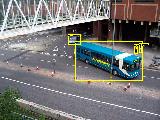
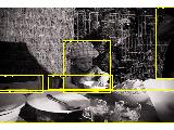
  2. Detection: Predicting the bounding box and label of each object from the twenty target classes in the test image.
    20 classes
    aeroplane bicycle bird boat bottle bus car cat chair cow
    dining table dog horse motorbike person potted plant sheep sofa train tv/monitor

Participants may enter either (or both) of these competitions, and can choose to tackle any (or all) of the twenty object classes. The challenge allows for two approaches to each of the competitions:

  1. Participants may use systems built or trained using any methods or data excluding the provided test sets.
  2. Systems are to be built or trained using only the provided training/validation data.

The intention in the first case is to establish just what level of success can currently be achieved on these problems and by what method; in the second case the intention is to establish which method is most successful given a specified training set.

Segmentation Competition

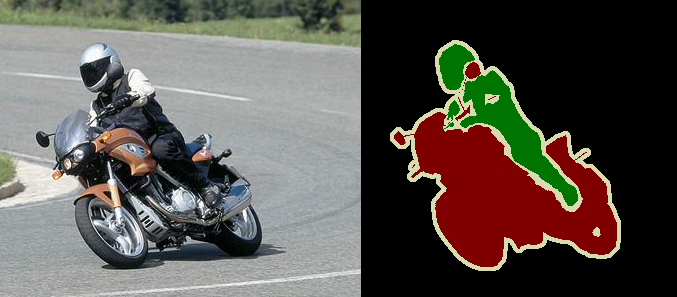
  • Segmentation: Generating pixel-wise segmentations giving the class of the object visible at each pixel, or “background” otherwise.
    Image Objects Class

Person Layout Taster Competition

  • Person Layout: Predicting the bounding box and label of each part of a person (head, hands, feet).
    Image Person Layout

Data

To download the training/validation data, see the development kit.

The training data provided consists of a set of images; each image has an annotation file giving a bounding box and object class label for each object in one of the twenty classes present in the image. Note that multiple objects from multiple classes may be present in the same image. Some example images can be viewed online. A subset of images are also annotated with pixel-wise segmentation of each object present, to support the segmentation competition. Some segmentation examples can be viewed online.

Annotation was performed according to a set of guidelines distributed to all annotators.

The data will be made available in two stages; in the first stage, a development kit will be released consisting of training and validation data, plus evaluation software (written in MATLAB). One purpose of the validation set is to demonstrate how the evaluation software works ahead of the competition submission.

In the second stage, the test set will be made available for the actual competition. As in the VOC2008 challenge, no ground truth for the test data will be released.

The data has been split into 50% for training/validation and 50% for testing. The distributions of images and objects by class are approximately equal across the training/validation and test sets. In total there are 14,743 images. Further statistics are online.

Example images

Example images and the corresponding annotation for the classification/detection/segmentation tasks, and and person layout taster can be viewed online:

Development Kit

The development kit consists of the training/validation data, MATLAB code for reading the annotation data, support files, and example implementations for each competition.

Test Data

The test data is now available. Note that the only annotation in the data is for the layout taster challenge – disjoint from the main challenge. As in 2008, there are no current plans to release full annotation – evaluation of results will be provided by the organizers.

The test data can now be downloaded from the evaluation server. You can also use the evaluation server to evaluate your method on the test data.

Useful Software

Below is a list of software you may find useful, contributed by participants to previous challenges.

Timetable

  • 15 May 2009: Development kit (training and validation data plus evaluation software) made available.
  • 15 June 2009: Test set made available.
  • 14 September 2009 (extended). Deadline for submission of results. There will be no further extensions.
  • 3 October 2009: Workshop in assocation with ICCV 2009, Kyoto, Japan.

Submission of Results

Participants are expected to submit a single set of results per method employed. Participants who have investigated several algorithms may submit one result per method. Changes in algorithm parameters do not constitute a different method – all parameter tuning must be conducted using the training and validation data alone.

Results must be submitted using the automated evaluation server:

It is essential that your results files are in the correct format. Details of the required file formats for submitted results can be found in the development kit documentation. The results files should be collected in a single archive file (tar/tgz/tar.gz). An example of the correct format is available:

The format of your results must match that specified in the development kit and in the example file, including both file names and directory structure. If you are not entering a particular competition, just omit the corresponding files.

Participants submitting results for several different methods (noting the definition of different methods above) should produce a separate archive for each method.

In addition to the results files, participants will need to additionally specify:

  • contact details and affiliation
  • list of contributors
  • brief description of the method

If you would like to submit a more detailed description of your method, for example a relevant publication, this can be included in the results archive.

Prizes

The following prizes were announced at the challenge workshop:

Classification
Winner: NEC/UIUC
Yihong Gong, Fengjun Lv, Jinjun Wang, Chen Wu, Wei Xu, Jianchao Yang, Kai Yu, Xi Zhou, Thomas Huang
NEC Laboratories America; University of Illinois at Urbana-Champaign
Honourable mentions: UVA/SURREY
Koen van de Sande, Fei Yan, Atif Tahir, Jasper Uijlings, Mark Barnard, Hongping Cai, Theo Gevers, Arnold Smeulders, Krystian Mikolajczyk, Josef Kittler
University of Amsterdam; University of SurreyCVC
Fahad Shahbaz Khan, Joost van de Weijer, Andrew Bagdanov, Noha Elfiky, David Rojas, Marco Pedersoli, Xavier Boix, Pep Gonfaus, Hany salahEldeen, Robert Benavente, Jordi Gonzalez, Maria Vanrell
Computer Vision Centre Barcelona
Detection
Joint Winners: UoC/TTI Chicago
Pedro Felzenszwalb, Ross Girshick, David McAllester
University of Chicago; Toyota Technological Institute at ChicagoOxford/MSR India
Andrea Vedaldi, Varun Gulshan, Manik Varma, Andrew Zisserman
University of Oxford; Microsoft Research India
Segmentation
Winner: Bonn
Joao Carreira, Fuxin Li, Cristian Sminchisescu
University of Bonn
Runner-up: CVC
Xavier Boix, Josep Maria Gonfaus, Fahad Kahn, Joost van de Weijer, Andrew Bagdanov, Marco Pedersoli, Jordi Gonzalez, Joan Serrat
Computer Vision Center Barcelona

Publication Policy

The main mechanism for dissemination of the results will be the challenge webpage.

The detailed output of each submitted method will be published online e.g. per-image confidence for the classification task, and bounding boxes for the detection task. The intention is to assist others in the community in carrying out detailed analysis and comparison with their own methods. The published results will not be anonymous – by submitting results, participants are agreeing to have their results shared online.

Citation

If you make use of the VOC2009 data, please cite the following reference (to be prepared after the challenge workshop) in any publications:

@misc{pascal-voc-2009,
	author = "Everingham, M. and Van~Gool, L. and Williams, C. K. I. and Winn, J. and Zisserman, A.",
	title = "The {PASCAL} {V}isual {O}bject {C}lasses {C}hallenge 2009 {(VOC2009)} {R}esults",
	howpublished = "http://www.pascal-network.org/challenges/VOC/voc2009/workshop/index.html"}	

Database Rights

The VOC2009 data includes images obtained from the “flickr” website. Use of these images must respect the corresponding terms of use:

For the purposes of the challenge, the identity of the images in the database, e.g. source and name of owner, has been obscured. Details of the contributor of each image can be found in the annotation to be included in the final release of the data, after completion of the challenge. Any queries about the use or ownership of the data should be addressed to the organizers.

Organizers

  • Mark Everingham (University of Leeds), me@comp.leeds.ac.uk
  • Luc van Gool (ETHZ, Zurich)
  • Chris Williams (University of Edinburgh)
  • John Winn (Microsoft Research Cambridge)
  • Andrew Zisserman (University of Oxford)

Acknowledgements

We gratefully acknowledge the following, who spent many long hours providing annotation for the VOC2009 database: Jan Hendrik Becker, Patrick Buehler, Kian Ming Adam Chai, Miha Drenik, Chris Engels, Hedi Harzallah, Nicolas Heess, Sam Johnson, Markus Mathias, Alastair Moore, Maria-Elena Nilsback, Patrick Ott, Florian Schroff, Alexander Sorokin, Paul Sturgess, David Tingdahl. We also thank Andrea Vedaldi for additional assistance.

The objective of the Challenge is to design a statistical machine learning algorithm that discovers which morphemes (smallest individually meaningful units of language) words consist of. Ideally, these are basic vocabulary units suitable for different tasks, such as text understanding, machine translation, information retrieval, and statistical language modeling.

The scientific goals are:

  • To learn of the phenomena underlying word construction in natural languages
  • To discover approaches suitable for a wide range of languages
  • To advance machine learning methodology

Morpho Challenge 2009 is a follow-up to our previous Morpho Challenge 2005, 2007 and 2008. The task of Morpho Challenge 2009 is similar to the Morpho Challenge 2008, where the aim was to find the morpheme analysis of the word forms in the data. For this challenge, new Machine Translation tasks are added (from Finnish to English and from German to English) to evaluate the performance of the morpheme analysis.

Participation in the previous challenges is by no means a prerequisite for participation in Morpho Challenge 2009. Everyone is welcome and we hope to attract many participating teams. The results will be presented in a workshop. Please read the rules and see the schedule. The datasets are available for download. Submit your analyses (result files) by sending them by email to the organizers, or by indicating a location where the organizers can download your files. Remember also to describe your algorithm in a paper. Please read the formatting instructions in rules.

If you plan to participate in Morpho Challenge, please contact the organizers using the email address in contact and ask to be added in our mailing list. We will use this mailing list to provide news about the tasks, data and evaluations.

The results from the evaluation runs are now in the Results page.
The Workshop was held in September 30, 2009

References

Mathias Creutz and Krista Lagus (2005). Unsupervised Morpheme Segmentation and Morphology Induction from Text Corpora Using Morfessor 1.0. Publications in Computer and Information Science, Report A81, Helsinki University of Technology, March.
[ Article (PDF) ]Teemu Hirsimäki, Mathias Creutz, Vesa Siivola, Mikko Kurimo, Janne Pylkkönen, and Sami Virpioja (2006). Unlimited vocabulary speech recognition with morph language models applied to Finnish.Computer Speech and Language, Volume 20, Issue 4, October, pages 515–541.
[ Article (PDF) ]

Sami Virpioja, Jaakko J. Väyrynen, Mathias Creutz, and Markus Sadeniemi (2007). Morphology-aware statistical machine translation based on morphs induced in an unsupervised manner. In Proceedings of the Machine Translation Summit XI, pages 491–498.
[ Article (PDF) ]

Mikko Kurimo and Matti Varjokallio (2008). Unsupervised morpheme analysis evaluation by a comparison to a linguistic Gold Standard – Morpho Challenge 2008. In Working Notes for the CLEF 2008 Workshop.
[ Article (PDF) ]

Mikko Kurimo and Ville Turunen (2008). Unsupervised morpheme analysis evaluation by IR experiments – Morpho Challenge 2008. In Working Notes for the CLEF 2008 Workshop.
[ Article (PDF) ]

Rules

Submission of large data files

Send an email to the organizers morphochallenge2008<>mail.cis.hut.fi and tell where they can download the data files. Small data files (but not larger than a few MBs) can be emailed directly. Please, follow carefully the format of the result files described in datasets.

Acceptance

The organizers retain all rights to the Challenge data, which is given to the participants for use in this challenge only. The organizers may use the data submitted to the Challenge freely, without restrictions.

Eligibility

Anyone is allowed to participate. A participant may be either a single person or a group. A single person can participate in at most two groups. A participant is allowed to submit at most three different solutions, where each solution corresponds to a particular morpheme analysis method. Each of these methods may naturally be applied to each of the test languages. If a participant submits more than three solutions, the organizers decide which of the three will be accepted.

Test languages

Data sets are provided for five languages: Arabic, English, Finnish, German and Turkish. Participants are encouraged to apply their algorithm to all of these test languages, but are free to leave some languages out, if they wish to do so.

(New languages may be added, if interested co-organizers, suitable data and evaluation analyses become available in time.)

Task

The task is to develop a system that conducts unsupervised morpheme analysis for every word form contained in a word list supplied by the organizers for each test language.

The participants will be pointed to corpora in which the words occur, so that the algorithms may utilize information about word context.

Solutions, in which a large number of parameters must be “tweaked” separately for each test language, are of little interest. This challenge aims at the unsupervised (or very minimally supervised) morpheme analysis of words. The abstracts submitted by the participants must contain clear descriptions of which steps of supervision or parameter optimization are involved in the algorithms.

Competitions

The segmentations will be evaluated in three complementary ways:

  • Competition 1: The proposed morpheme analyses will be compared to a linguistic “gold standard”.
  • Competition 2: Information retrieval (IR) experiments will be performed, where the words in the documents and queries will be replaced by their proposed morpheme representations. The search will then be based on morphemes instead of words.
  • Competition 3: Machine Translation (MT) model is trained, where the words in the source language documents will be replaced by their proposed morpheme representations. The words in the source language evaluation data will then also be replaced by their proposed morpheme representations and the translation will be based on morphemes instead of words.

Competition 1 will include all five test languages. Winners will be selected separately for each language. As a performance measure, the F-measure of accuracy of suggested morpheme analyses is utilized. Should two solutions produce the same F-measure, the one with higher precision will win.

Competition 2 will include three of the test languages. The organizers will perform the IR experiments based on the morpheme analyses submitted by the participants.

Competition 3 will include two of the test languages. Translation will be done from the test language to English. The organizers will train the translation models and perform the evaluation of the translations using an automatic metric such as BLEU.

Workshop and publication

All good results will be acknowledged with fame and glory. Presentations for the challenge workshop will be selected by the organizers based on the results and a paper of at most 10 pages describing the algorithm and the data submission. However, all groups who have submitted results and a paper are welcome to participate in the workshop to listen to the talks and join the discussions.

Workshop papers

For your paper submission (due August 15), please use the single-column CLEF 2007 Notebook Proceedings format. Here are a sample PDF file and a template Latex document. Email your paper submission to the organizers.
Formatting instructions:

size: A4
format: pdf (if difficult, ps or MS Word (rtf) are acceptable) Do NOT lock the pdf file.
borders: top, left right 2.5 cm ; bottom 3 cm
text size: 16 x 24 cm
length: 10 pages maximum
title: Times 14 pt bold centered
author(s): Times 10 pt centered
abstract: Times 10 pt justified
ACM Categories and Subject Descriptors: Times 10 pt left aligned
Free Keywords: Times 10 pt left aligned
body text: Times 10 pt justified
Section Headings: Times 12 pt bold left aligned
Emphasis: Times 10 pt italic

Arbitration

In the case of disagreement the organizers will decide the final interpretation of the rules.

Competition 1

NEW: The evaluation measures of competition 1 are updated for Morpho Challenge 2009. Some bugs related to the handling of alternative analyses are fixed from the scripts, and points are now measured as one per word, not one per word pair. The new evaluation scripts are now available:


The old scripts are found from Challenge 2008.

In Competition 1, for each language, the morpheme analyses proposed by the participants’ algorithm will be compared against a linguistic gold standard. Samples of the gold standards used are available for download on the datasets page.

Since the task at hand involves unsupervised learning, it cannot be expected that the algorithm comes up with morpheme labels that exactly correspond to the ones designed by linguists. That is, no direct comparison will take place between labels as such (the labels in the proposed analyses vs. labels in the gold standard). What can be expected, however, is that two word forms that contain the same morpheme according to the participants’ algorithm also have a morpheme in common according to the gold standard. For instance, in the English gold standard, the words “foot” and “feet” both contain the morpheme “foot_N”. It is thus desirable that also the participants’ algorithm discovers a morpheme that occurs in both these word forms (be it called “FOOT”, “morpheme784”, “foot” or something else).

In practice, the evaluation will take place by sampling a large number of word pairs, such that both words in the pair have at least one morpheme in common. As the evaluation measure, we will use F-measure, which is the harmonic mean of Precision and Recall:

F-measure = 1/(1/Precision + 1/Recall).

Precision is here calculated as follows: A number of word forms will be randomly sampled from the result file provided by the participants; for each morpheme in these words, another word containing the same morpheme will be chosen from the result file by random (if such a word exists). We thus obtain a number of word pairs such that in each pair at least one morpheme is shared between the words in the pair. These pairs will be compared to the gold standard; a point is given for each word pair that really has a morpheme in common according to the gold standard. The maximum number of points for one sampled word is normalized to one. The total number of points is then divided by the total number of sampled words.

For instance, assume that the proposed analysis of the English word “abyss” is: “abys +s”. Two word pairs are formed: Say that “abyss” happens to share the morpheme “abys” with the word “abysses”; we thus obtain the word pair “abyss – abysses”. Also assume that “abyss” shares the morpheme “+s” with the word “mountains”; this produces the pair “abyss – mountains”. Now, according to the gold standard the correct analyses of these words are: “abyss_N”, “abyss_N +PL”, “mountain_N +PL”, respectively. The pair “abyss – abysses” is correct (common morpheme: “abyss_N”), but the pair “abyss – mountain” is incorrect (no morpheme in common). Precision for the word “abyss” is thus 1/2 = 50%.

Recall is calculated analogously to precision: A number of word forms are randomly sampled from the gold standard file; for each morpheme in these words, another word containing the same morpheme will be chosen from the gold standard by random (if such a word exists). The word pairs are then compared to the analyses provided by the participants; a point is given for each sampled word pair that has a morpheme in common also in the analyses proposed by the participants’ algorithm. Points per word is normalized to one and the total number of points is divided by the total number of words.

For words that have several alternative analyses, as well as for word pairs that have more than one morpheme in common, normalization of the points is carried out. In short, an equal weight is given for each alternative analysis, as well as each word pair in an analysis. E.g., if a word has three alternative analyses, the first analysis has four morphemes, and the first word pair in that analysis has two morphemes in common, each of the two common morphemes will amount to 1/3*1/4*1/2=1/24 of the one point available for that word.

Evaluation of a sample (development test set)

You can evaluate your morphological analyses against the available gold standards (separately for each test language). The program to use for this is the Perl script: eval_morphemes_v2.pl. The evaluation program is invoked as follows:

eval_morphemes_v2.pl [-trace] wordpairsfile_goldstd wordpairsfile_result goldstdfile resultfile

Four files are given as arguments to eval_morphemes_v2.pl:

  1. wordpairsfile_goldstd: this is the “random word pairs file” available for download on the datasets page. This file is needed in the calculation of an estimate of the recall of the proposed morpheme analyses.
  2. wordpairsfile_result: this file has to be generated using another program (see below). It is needed in the calculation of a rough estimate of the precision of the proposed morpheme analyses.
  3. goldstdfile:this is the sample of the gold standard available for download on the datasets page. This file contains the correct morpheme analyses for circa 500 words.
  4. resultfile: this is the result file that your algorithm produces, i.e., a list of words and their proposed morpheme analyses.

The -trace argument is optional and produces output for every evaluated word separately. Regardless of the status of the trace argument, the evaluation program produces output of the following kind:

PART0. Precision: 69.00% (96/139); non-affixes: 81.55% (51/63); affixes: 58.73% (45/76)
PART0. Recall:    25.59% (142/556); non-affixes: 49.78% (105/211); affixes: 10.78% (37/345)
PART0. F-measure: 37.33%; non-affixes: 61.82%; affixes: 18.22%
#
TOTAL. Precision: 69.00%; non-affixes: 81.55%; affixes: 58.73%
TOTAL. Recall:    25.59%; non-affixes: 49.78%; affixes: 10.78%
TOTAL. F-measure: 37.33%; non-affixes: 61.82%; affixes: 18.22%

Note that results are displayed for partition 0 (PART0) and for the entire data (TOTAL). The total scores are here the same as the scores of PART0, since there is only one partition. It is, however, possible to split the data into several partitions and compute results for each partition separately. The overall scores are then calculated as the mean over the partitions. Splitting into partitions is a feature reserved for the final evaluation, when we will assess the statistical significance of the differences between the participants’ algorithms.

The figures that count in the final evaluation are the first precision, recall, and F-measure values on the TOTAL lines. These values pertain to all morphemes, but there are also separate statistics for morphemes classified as non-affixes vs. affixes. What counts as an affix is a morpheme with a label starting with a plus sign, e.g., “+PL”, “+PAST”. This naming convention is applied in the gold standard, which means that you do not have to do anything in order to get the non-affixes/affixes statistics right as far as recall is concerned. However, if you want the same kind of information also for precision, your algorithm must have a means of discovering which morphemes are likely affixes and tag these morphemes with an initial plus sign. Note that it is fully up to you whether you do this or not; it will not affect your position in the competition in any way.

Sampling word pairs for the calculation of an estimate of the precision

In order to get an estimate of the precision of the algorithm, you need to provide the evaluation script eval_morphemes_v2.pl with a file containing word pairs sampled from your result file. Unfortunately, the estimate is likely to be fairly rough. The reason for this is that you do not have the entire gold standard at your disposal. Thus, if you sample pairs of words that are not included in the 500-word gold standard that you can access, it is impossible to know whether the proposed morphemes are correct or not. What you can do, however, is to make sure that each word that goes into a word pair actually does occur in the 500-word gold standard sample. The problem here is that your algorithm might not propose that many common morphemes for the words within this limited set, and thus the estimate will be based on rather few observations.

Anyway, this is how to do it: First, make a list of relevant words, that is, words that are present in the gold standard sample available:

cut -f1 goldstdfile > relevantwordsfile

Then sample word pairs for 100 words selected by random from your results file:

sample_word_pairs_v2.pl -refwords relevantwordsfile < resultfile > wordpairsfile_result

The necessary Perl program is sample_word_pairs_v2.pl. The output file wordpairsfile_result is used as input to eval_morphemes_v2.pl (see above).

Competition 2

Competition 2 does not necessarily require any extra effort by the participants. The organizers will use the analyses provided by the participants in information retrieval experiments. Data from CLEF will be used.
However, those participants who wish to submit morpheme analysis for words in their actual context (competition 2b), please contact the organizers for more information how to register to CLEF to obtain the full texts.

In the competition 2 (and 2b) the words in the queries and documents will be replaced by the corresponding morpheme analyses provided by the participants. We will perform the IR evaluation using the state-of-the-art Okapi (BM25) retrieval method (the latest version of the freely available LEMUR toolkit. The most common morphemes in each participant’s submission will be left out from the index. The size of this stoplist will be proportional to the amount of the text data in each language and the stoplist size will be the same for each participant’s submission. The evaluation criterion will be Uninterpolated Average Precision. The segmentation with the highest Average Precision will win. The winner is selected separately for competitions 2 and 2b in each language.

Competition 3

In competition 3, the morpheme analyses proposed by the participants’ algorithm will be evaluated in a statistical machine translation (SMT) framework. The translation models will be trained to translate from a morphologically complex source language to English. The words of the source language will be replaced by their morpheme analyses before training. The translations from this morpheme-to-word model will be combined with translations from a standard word-to-word translation model. For all models, we will use a state-of-the-art phrase-based SMT system. Evaluation of the translations will be performed by applying an automatic metric such as BLEU on a held-out test set.

Data is from the Europarl corpus. The participants should apply their algorithms to the list of the word forms in the corpus. It is also possible to use the context information of the words by downloading the full corpus. (See datasets for details.)

This workshop presented and discussed the results of the PASCAL Visual Object Classes Challenge (VOC2008). As in previous years’ challenges there are two main competitions, one testing image classification (“does the image contain an instance of this class?”), and one testing object detection (“provide a bounding box for each instance of the class, if any”). In addition there are two ‘taster’ competitions: the first evaluates the object layout in more detail (“detect the hands, feet etc for a person”), the second evaluates object segmentation at the pixel level.

A new database has been prepared consisting of 20 classes with around 25000 annotated instances in total. The images are obtained from flickr. The classes include people, cats, dogs, cars, motorbikes, bottles and sofas. The annotation includes a rectangular bounding box and flags to indicate pose and level of difficulty.

Organizers

  • Mark Everingham (University of Leeds), me@comp.leeds.ac.uk
  • Luc van Gool (ETHZ, Zurich)
  • Chris Williams (University of Edinburgh)
  • John Winn (Microsoft Research Cambridge)
  • Andrew Zisserman (University of Oxford)

Challenge Rules

  • Conditions of participation: Anybody who complies with the rules of the challenge is welcome to participate. There are two modes of participation:
    • As a data donor by making an entry in the Repository.
    • As a problem solver by submitting results on at least one of the proposed tasks.
  • Dissemination: The challenge results will be presented at a NIPS 2008 conference workshop, December 12, 2008. To present at the workshop, abstracts must be submitted before October 24, 2008 to causality@clopinet.com. Participants are not required to attend the workshop and the workshop is open to non-challenge participants. The proceedings of the competition will be published by the Journal of Machine Learning Research (JMLR).
  • Anonymity: The participants who do not submit a paper to the workshop can elect to remain anonymous. Their results will be published, but their name will remain confidential.
  • Tasks: A number of datasets on which tasks have been defined are available, see the Task page. More tasks will be added from time to time, if new data are donated. Data donated show up immediately in the Repository, but they become part of the challenge only after beeing reviewed by the organizers, who then add them to the Task page. To be informed of task updates, request to be added to our mailing list by sending email to causality@clopinet.com.
  • Milestone and final results: Results must be submitted between the start and the termination of the challenge. The challenge starts on September 15, 2008 and is scheduled to terminate on November 12, November 19, 2008. Each participating team is allowed to submit one set of results per task for the final evaluation. If more than one set of results is submitted, the last one will be taken into account. The results of the final evaluation will be publicly released at the workshop. In addition, optionally, each participating team may submit one set of results before October 15, 2008 to be part of the milestone evaluation, whose results will be publicly but anonymously released.
  • Submission method: The results on each task must be sent to the designated contact person, see the Task page. In case of problem, send email to causality@clopinet.com.
  • Evaluation and rewards: To compete towards the prizes, the participants must submit a 6-page paper describing their donated dataset (if they entered as a donor) or their task-solving method(s) and result(s) (if they entered as a solver), before November 21, 2008, to causality@clopinet.com (A sample paper and a Latex style file are provided). The challenge participants must append their fact sheet to their paper, see template provided in Latex (sample paper appendix), MS Word, or Acrobat formats. Each participant is allowed to submit several papers, if they address or propose distinct problems. The contributions of the participants will be evaluated by the organizers on the basis of their challenge performance results, the post-challenge tests (see reproducibility), AND the paper, using the following criteria: Performance in challenge and general Usefulness, Novelty and Originality, Sanity, Insight, Reproducibility, and Clarity of presentation. The data donors may provide solutions to their own problems, however such contribution will not count towards winning the prizes. Close collaborators of data donors having access to information, which may give them an unfair advantage, should disclose this fact to the organizers. The best papers will be selected for presentation at the workshop and several Prizes will be awarded.
  • Reproducibility: Participation is not conditioned on delivering your code nor publishing your methods. However, we will ask the top ranking participants to voluntarily cooperate to reproduce their results. This will include filling out a fact sheet about their methods (get template in Latex, MS Word, or Acrobat formats) and eventually participating to post-challenge tests and sending us their code, including the source code. The outcome of our attempt to reproduce your results will be published and add credibility to your results.

Challenge Tasks

The Pot-luck challenge datasets are a selection of the Repository datasets. Presently, we propose the following tasks:

  • CYTO: Causal Protein-Signaling Networks in human T cells. The task is to learn a protein signaling network from multicolor flow cytometry data, recording the molecular activity of 11 proteins. There is on average 800 samples per experimental condition, corresponding to various perturbations of the system (manipulations). The authors used a Bayesian network approach and demonstrated that they recover most of the known signaling network structure, while discovering some new hypothetical regulations (causal relationships). The tasks suggested to the challenge participants include reproducing the results of the paper and finding a method to assess the confidence of the causal relationships uncovered. The evaluation is via submitted papers.
  • LOCANET: LOcal CAusal NETwork We regroup under the name LOCANET a number of tasks consisting in finding the local causal structure around a given target variable (depth 3 network). The following datasets lend themselves to performing such a task: REGED, CINA, SIDO, MARTI. The results are evaluated by the organizers upon submition of the local structure in a designated format. In addition, the toy dataset LUCAS can be used for self evaluation.
  • PROMO: Simple causal effects in time series. The task is to identify which promotions affect sales. This is an artificial dataset of about 1000 promotion variables and 100 product sales. The goal is to predict a 1000×100 boolean influence matrix, indicating for each (i,j) element whether the ith promotion has a causal influence of the sales of the jth product. Data is provided as time series, with a daily value for each variable for three years (i.e., 1095 days). The ground truth for the influence matrix is provided, so the participants can self-evaluate their results, and submit a paper to compete for the prizes.
  • SIGNET: Abscisic Acid Signaling Network. The objective is to determine the set of 43 boolean rules that describe the interactions of the nodes within a plant signaling network. The dataset includes 300 separate boolean pseudodynamic simulations of the true rules, using an asynchronous update scheme. This is an artificial dataset inspired by a real biological system. The results are evaluated by the contact person upon submission of the results in a designated format.
  • TIED: Target Information Equivalent Dataset. This is an artificial simulated dataset constructed to illustrate that there may be many minimal sets of features with optimal predictivity (i.e., Markov boundaries) and likewise many sets of features that are statistically indistinguishable from the set of direct causes and direct effects of the target. The tasks suggested include determining all statistically undistinguishable sets of direct causes and effects, or Markov boundaries of the target variable, and predicting the target variable on test data. The results are evaluated by the contact person upon submission of the results in a designated format.

Note that the participants are ultimately judged on their paper(s). For each dataset, the tasks proposed are only suggestions. The participants are invited to use the data is a creative way and propose their own task(s).

New: tasks proposed by participants

October 30: The following tasks proposed by participants are now included in the challenge.

  • CauseEffectPairs: Distinguishing between cause and effect. The data set consists of 8 N x 2 matrices, each representing a cause-effect pair and the task is to identify which variable is the cause and which one the effect. The origin of the data is hidden for the participants but known to the organizers. The data sets are chosen such that we expect common agreement on which one is the cause and which one the effect. Even though part of the statistical dependences may also be due to hidden common causes, common sense tells us that there is a significant cause-effect-relation.
  • STEMMATOLOGY: Computer-assisted stemmatology. Stemmatology (a.k.a. stemmatics) studies relations among different variants of a document that have been gradually built from an original text by copying and modifying earlier versions. The aim of such study is to reconstruct the family tree (causal graph) of the variants. We provide a dataset to evaluate methods for computer-assisted stemmatology. The ground truth is provided, as are evaluation criteria to allow the ranking of the results of different methods. We hope this will facilitate the development of novel approaches, including but not restricted to hierarchical clustering, graphical modeling, link analysis, phylogenetics, string-matching, etc.

Data donation

Another way to participate in the challenge is to donate data. You will need to first Register . Then you will need to fill out a form to Deposit your data.Our repository does not actually store data, it points to a web page YOUR_DATA.html, which you maintain, and from which your data is accessible. If you do not have a web server allowing you to maintain a web page for your data, you may use the UCI Machine Learning Repository, which physically archives data or contact us at causality@clopinet.com.

Your entry can be edited after submission, but we recommend that you prepare your submission in a text file before filling out the form.

Tips to fill out your submission form:

  • Contact name/URL: Select a person, which will be available to answer questions and evaluate results.
  • Resource type: Choose “data” (eventually you can submit a generative model of data, then choose “model”).
  • Resource name: A short easy-to-memorize acronym.
  • Resource url: This is the web page you maintain YOUR_DATA.html.
  • Title: A title describing your dataset.
  • Authors: A comma separated list of authors.
  • Key facts: Data dimensions (number of variables, number of entries), variable types, missing data, etc.
  • Keywords: A comma separated list of keywords.
  • Abstract: A brief description of your dataset and the task to be solved, including:
    • Background.
    • Data description.
    • Task description.
    • Result format.
    • Result submission method.
    • Evaluation metrics.
    • Suggestion of other tasks.

    If you provide a web page YOUR_DATA.html, more details can be given there.

  • Supplements 1, 2, and 3: Use these fields to provide a direct pointer to a zip archive to download data, a published paper or a report on the data, some slides, etc.


With the exceptional increase in computing power, storage capacity and network bandwidth of the past decades, ever growing datasets are collected in fields such as bioinformatics (Splice Sites, Gene Boundaries, etc), IT-security (Network traffic) or Text-Classification (Spam vs. Non-Spam), to name but a few. While the data size growth leaves computational methods as the only viable way of dealing with data, it poses new challenges to ML methods.

This PASCAL Challenge is concerned with the scalability and efficiency of existing ML approaches with respect to computational, memory or communication resources, e.g. resulting from a high algorithmic complexity, from the size or dimensionality of the data set, and from the trade-off between distributed resolution and communication costs.

Indeed many comparisons are presented in the literature; however, these usually focus on assessing a few algorithms, or considering a few datasets; further, they most usually involve different evaluation criteria, model parameters and stopping conditions. As a result it is difficult to determine how does a method behave and compare with the other ones in terms of test error, training time and memory requirements, which are the practically relevant criteria.

We are therefore organizing a competition, that is designed to be fair and enables a direct comparison of current large scale classifiers aimed at answering the question “Which learning method is the most accurate given limited resources?”. To this end we provide a generic evaluation framework tailored to the specifics of the competing methods. Providing a wide range of datasets, each of which having specific properties we propose to evaluate the methods based on performance figures, displaying training time vs. test error, dataset size vs. test error and dataset size vs. training time.

General

The overall goal is to develop a 2-class classifier such that it achieves a low error in the shortest possible time using as few datapoints as possible.

  • All participants are required to identify themselves with a login name, full name and a valid Email address. Your email address will not be made public and is only used for registration and announcements (test dataset release, workshop date, awards). The login name and your full name will appear on the evaluation page.
  • In order to be included in the final evaluation process, every participant should compete on at least five datasets in a single track, i.e. submit results on the validation/test set of five problems for the Wild track, or for one of the SVM tracks.
  • Every participant will provide computational time (training time and separately time required to do predictions for the optimal model-parameter setting excluding data loading times) associated to every submission, accompanied with an estimation of their computing power. This estimation is provided by running a calibration program provided by the challenge organizers.
  • In order to assess more precisely how the accuracy depends on the computational time, every participant is kindly asked to provide the predictions obtained for various fractions of the total computational time T, on the biggest dataset he or she will consider. Preferred fractions: T/10,T/9…,T
  • After the end of the competition, every participant will provide an extended abstract (4 pages) describing the algorithm.
  • All participants will be requested to provide executable or source code, allowing to re-run the algorithm under the same computing conditions, for a later timing re-calibration and re-run of the top-ten methods.

In order to fairly assess the performances of the SVM-QP solvers, the participants to the SVM tracks are asked to comply with two requirements:

  • NO DATA PREPARATION ALLOWED (no feature construction, no feature selection, …).
  • NO PARAMETER TUNING ALLOWED (penalization factor C, and Gaussian kernel radius tau, are set to a prescribed value)

Challenge Tasks

The overall goal is to tune your method such that achieves a low test error measured by the area over the precision recall curve in the shortest possible time and using as few datapoints as possible.

Wild Competition Track

In this track you are free to do anything that leads to more efficient, more accurate methods, e.g. perform feature selection, find effective data representations, use efficient program-code, tune the core algorithm etc. It may be beneficial to use the raw data representation (described below). For each dataset your method competes in you are requested to:

  • Train on 10^[2,3,4,5,6,7] and the maximum number of available datapoints. If your method cannot cope with all dataset sizes you are allowed to skip over too large datasets. For all of the training sessions the training time and time required to compute test outputs has to be recorded.
  • Additionally for the biggest dataset your method can deal with, we ask you to provide ten intermediate time/output-recordings. These can be obtained, by for example training twice and computing time and output after time T/10, T/9, …T (where T is the overall training time). Do not forget to include test-times in each of the recordings.

SVM Tracks

To allow for a comparison w.r.t. to non-SVM solvers, all SVM methods are required to compete in both tracks and therefore for SVMs step 1 is to attack the wild-track task. In addition to what has to be done in the wild track we ask you to do the following experiments.

  1. To measure convergence speed, we ask you to re-do the wild-track experiment for a fixed setting of C=0.01, epsilon=0.01 (and rbf kernel width tau=10) but measuring primal objective only.
  2. To simulate model selection you are requested to train SVMs for different C and rbf-widths keeping epsilon=0.01 fixed, again only measuring objective value.

Here epsilon denotes the relative duality gap (obj_primal-obj_dual)/obj_primal<epsilon=0.01. If your solver has a different stopping condition, choose it reasonably, i.e. such that you expect it to have similar duality gap. While early stopping is OK it may hurt your method in evaluation: If the objective of your svm solver deviates too much from others, i.e. by more than 5% (your_obj-obj_min)/your_obj<0.05, it will get low scores. Note that you have to use the data representation obtained by running the svmlight-conversion script in the second part (model selection) of the experiment. The following values for C/rbf-width shall be used:

  • for the Linear SVM Track it is required to train SVMs for Cs=[0.0001, 0.001, 0.01, 0.1, 1, 10]
  • for the RBF Kernel SVM Track it is required to train SVMs for fixed C=0.01 and tau=[0.01, 0.1, 1, 10, 100, 1000], whereK(x,y)= exp(-||x-y||^2 / tau).

Objective values are computed as follows:

  • for the Linear SVM Track
  • for the RBF Kernel SVM Track

Finally, if possible please include all parameters, rbf-tau, epsilon, SVM-C for all experiments in the result file.

Parallel Track

The recent paradigm shift of learning from single to multi-core shared memory architectures is the focus of the parallel track. For the parallel track methods have to be trained on 8 CPUs following the rules outlined in the wild track. To assess the parallelization quality, we in addition ask participants to train their method using 1,2,4,8 CPUs on the biggest dataset they can process. Note that the evaluation criteria are specifically tuned to parallel shared memory algorithms, i.e. instead of training time on each CPU you should measure wall-clock-time (including data loading time). In addition data loading time must be specified in a separate field.

Datasets

The raw datasets can be downloaded from ftp://largescale.ml.tu-berlin.de/largescale. The provided script convert.py may be used to obtain a simple (not necessary optimal) feature representation in svm-light format.

Overview of the Raw Datasets

Dataset Training Validation Dimensions Format Description
alpha 500000 100000 500
Files are in ascii format, where each line corresponds to 1 example,
i.e.

  val1 val2 ... valdim\n
  val1 val2 ... valdim\n
  ...
beta 500000 100000 500
gamma 500000 100000 500
delta 500000 100000 500
epsilon 500000 100000 2000
zeta 500000 100000 2000
fd 5469800 532400 900
  Files are binary, to obtain 1 example read 900 or 1156 bytes
  respectively (values 0..255)
ocr 3500000 670000 1156
dna 50000000 1000000 200
Files are ascii, each line contains a string of length 200 (symbols
ACGT), i.e.

  CATCATCGGTCAGTCGATCGAGCATC...A\n
  GTGTCATCGTATCGACTGTCAGCATC...T\n
  ...
webspam 350000 50000 variable
Files contains strings (webpages) separated with 0, i.e.
        html foo bar .../html\0

Submission Format

We provide an evaluation script that parses outputs and computes performance scores. We use this exact same script to do the live evaluation. It is suggested to run this script locally on a subset of the training data to test whether the submission format is correctly generated and to evaluate the results (note that the script can only be used on data where labels are available, e.g. subsets of the training data). It requires python-numpy and scipy to be installed. Additionally if matplotlib is installed, the performance figures will be drawn.

Additionally the data submission format is described below:

    • Wild Competition (download example submission)
              dataset_size0 -1 traintime0 testtime0 calibration0 objective C epsilon rfb-tau output0 output1 ...
              ...
              dataset_sizeN -1 traintimeN testtimeN calibrationN objective C epsilon rfb-tau output0 output1 ...
              dataset_sizeN index0 traintime0 testtime0 calibration0 objective C epsilon rfb-tau output0 output1 ...
              ...
              dataset_sizeN index9 traintime9 testtime0 calibration9 objective C epsilon rfb-tau output0 output1 ...
      
    • SVM Tracks (download example submission)A submission to the SVM track requires to take part in the wild competition, i.e. the submission file must start with the lines required for the wild competition. Then a single empty line announces the SVM-Track specific data:
      >a singly empty line here distinguishes wild from model specific track
              dataset_size0 -1 traintime0 testtime0 calibration0 objective C epsilon rfb-tau
              ...
              dataset_sizeN -1 traintimeN testtimeN calibrationN objective C epsilon rfb-tau
              dataset_sizeN index1 traintime1 testtime1 calibration1 objective C epsilon rfb-tau
              ...
              dataset_sizeN index9 traintime9 testtime0 calibration9 objective C epsilon rfb-tau
              dataset_sizeN -2 traintime0 testtime0 calibration0 objective C1 epsilon rfb-tau
              ...
              dataset_sizeN -2 traintimeK testtimeK calibration9 objective CK epsilon rfb-tau
      
      (or -3 and rbf-tau 1 ... K)


  • Parallel Track


A submission to the parallel track consists of two parts: The first one has the exact same syntax as the wild track (with time = wall-clock-time). The second part contains the 1,2,4,8 CPU experiment run on the biggest dataset (here C denotes the number of CPUs)

>a singly empty line here distinguishes wild from model specific track
        dataset_sizeN -4 walltimeN dataloadingtimeN calibrationN objective 1 epsilon rfb-tau
        dataset_sizeN -4 walltimeN dataloadingtimeN calibrationN objective 2 epsilon rfb-tau
        dataset_sizeN -4 walltimeN dataloadingtimeN calibrationN objective 4 epsilon rfb-tau
        dataset_sizeN -4 walltimeN dataloadingtimeN calibrationN objective 8 epsilon rfb-tau

Explanation of values (Column by Column)

  1. Dataset size – Values must match size of dataset or 10^[2,3,4,5,6,7]
  2. Index values of 0…9 (to distinguish values obtained while optimizing) only for the biggest dataset, -1 otherwise; for the SVM track -2 for the C experiment and -3 for the rbf-tau experiment
  3. Traintime – Time required for training (without data loading) in seconds / wall-clock time (including data loading) for the parallel track
  4. Testtime – Time required for applying the classifier to the validation/test data (without data loading) in seconds / data loading time for the parallel track
  5. Calibration – Score obtained using the provided calibration tool (values should be the same if run on the same machine)
  6. Method specific value: SVM Objective
  7. SVM-C / number of CPUs for the parallel track
  8. SVM-rbf-tau
  9. SVM epsilon
    • use 0 (for SVM Objective, SVM-C, SVM-rbf-tau, SVM epsilon) if not applicable
    • for SVM please fill in the different parameters, i.e. SVM objective, SVM-C, rbf-tau and stopping condition epsilon, as the meaning of epsilon may differ please explain in the description what epsilon stands for
    • for the linear svm track index -2 should be used when doing the experiment for C
    • for the gaussian svm track index -3 should be used when modifying rbf tau
  • The following values in columns 10-… must match the size of the validation/test set.

Assessment of the submissions

Different procedures will be considered depending on the track.

Wild Competition

For the Wild track, the ideal goal would be to determine the best algorithm in terms of learning accuracy, depending on the time budget allowed. Accordingly, the score of a participant is computed as the average rank of its contribution wrt the six scalar measures:

Time vs. Error This figure measures training time vs. area over the precision recall curve (aoPRC). It is obtained by displaying the different time budgets and their corresponding aoPRC on the biggest dataset. We compute the following scores based on that figure:

  • Minimum aoPRC
  • Area under Time vs. aoPRC Curve
  • The time t for which the aoPRC x falls below a threshold (x-overall_minimum_aoPRC)/x<0.05.
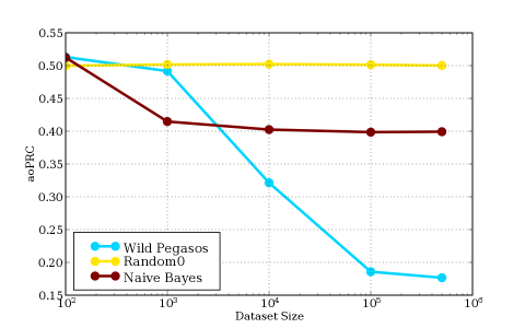
Size vs. Error This figure measures dataset size vs. area over the precision recall curve (aoPRC). It is obtained by displaying the different dataset sizes and their corresponding aoPRC that the methods achieve. We compute the following scores based on that figure:

  • Area under Size vs. aoPRC Curve
  • The size s for which the aoPRC x falls below a threshold (x-overall_minimum_aoPRC)/x<0.05.
Size vs Time This figure measures dataset size vs. training time. It is obtained by displaying the different dataset sizes and the corresponding training time that the methods achieve. We compute the following scores based on that figure:

  • Slope of the Curve b using a least squares fit to a*x^b.

SVM Tracks

For the SVM track, the point is to determine the best tradeoff between the computational effort and the learning accuracy. Accordingly, the score of a participant is computed as the average rank of its contribution wrt the five scalar measures

  • Minimal objective
  • Area under the Time vs. Objective Curve
  • Time to reach objective within 5% tolerance, i.e. minimal t for (t,obj) with (obj-overal_min_objective)/obj<0.05
  • Average Training Time for all C/Sigma
  • Computational Effort (scaling with dataset size)


Validation Results


Overall Ranking

Rank Score Submitter Title Date
1 4.40 chap – Olivier Chapelle Newton SVM 02.05.2008 20:57 CET
2 5.20 yahoo – Olivier Keerthi SDM SVM L2 19.06.2008 13:49 CET
3 5.60 yahoo – Olivier Keerthi SDM SVM L1 18.06.2008 19:28 CET
4 5.80 antoine – Antoine Bordes SgdQn 16.06.2008 14:21 CET
5 7.90 kristian – Kristian Woodsend IPM SVM 2 23.06.2008 15:10 CET
5 7.90 kristian – Kristian Woodsend Interior Point SVM 16.06.2008 21:56 CET
7 8.60 beaker – Gavin Cawley LR 19.06.2008 13:21 CET
8 9.90 ker2 – Porter Chang CTJ LSVM01 20.06.2008 03:31 CET
9 10.70 rofu – Rofu yu test 10.06.2008 16:31 CET
10 11.70 MB – Marc Boulle Averaging of Selective Naive Bayes Classifiers final 20.06.2008 12:06 CET
11 11.90 beaker – Gavin Cawley ORRR 12.06.2008 16:13 CET
11 11.90 rofu – Rofu yu liblinear 25.06.2008 11:57 CET
13 12.60 MB – Marc Boulle Averaging of Selective Naive Bayes Classifiers 27.05.2008 14:56 CET
14 14.00 garcke – Jochen Garcke AV SVM 02.06.2008 13:41 CET
15 14.10 aiiaSinica – Han-Shen Huang CTJ LSVM 19.06.2008 04:16 CET
16 14.70 fravoj – Vojtech Franc Random 18.02.2008 15:29 CET
17 15.20 beaker – Gavin Cawley WRRR 24.06.2008 13:12 CET
18 15.50 rofu – Rofu yu L1 13.06.2008 13:17 CET
19 16.30 antoine – Antoine Bordes LaRankConverged 13.06.2008 19:11 CET
20 17.20 beaker – Gavin Cawley ORRR Ensemble 15.06.2008 16:54 CET
21 17.40 ker2 – Porter Chang CTJ LSVM02 25.06.2008 14:38 CET
22 18.80 fravoj – Vojtech Franc ocas 25.06.2008 14:28 CET
22 18.80 antoine – Antoine Bordes Larank 13.06.2008 14:37 CET
24 19.20 beaker – Gavin Cawley rr 06.06.2008 21:14 CET
24 19.20 garcke – Jochen Garcke AV SVM single 25.06.2008 15:58 CET
26 19.30 aiiaSinica – Han-Shen Huang linearSVM01 11.06.2008 03:42 CET
26 19.30 xueqinz – Xueqin Zhang CHSVM 07.01.2009 01:27 CET
28 19.60 garcke – Jochen Garcke AV SVM 500k 10.06.2008 11:49 CET
28 19.60 garcke – Jochen Garcke AV SVM rbf track 23.06.2008 14:23 CET
30 19.70 fravoj – Vojtech Franc Stochastic SVM 18.02.2008 14:29 CET
31 20.30 aiiaSinica – Han-Shen Huang linearSVM03 16.06.2008 05:58 CET
32 20.40 rofu – Rofu yu Coordinate descent dual l1 linear svm 10.06.2008 15:21 CET
33 20.50 aiiaSinica – Han-Shen Huang sLsvm 17.06.2008 08:51 CET
34 20.70 ker2 – Porter Chang CTJsvm 21.01.2009 12:42 CET
35 20.80 aiiaSinica – Han-Shen Huang lsvm04 16.06.2008 06:57 CET
36 21.00 ker2 – Porter Chang anSGD 05.01.2009 08:21 CET
37 21.10 xueqinz – Xueqin Zhang CHSVM4 14.01.2009 06:13 CET
38 21.30 fravoj – Vojtech Franc random2 25.06.2008 14:48 CET
39 21.40 bernhardP – Bernhard Pfahringer Random model trees 11.06.2008 11:29 CET
40 21.70 fravoj – Vojtech Franc ocas new 26.02.2009 16:28 CET
41 21.80 beaker – Gavin Cawley LR3 31.07.2008 11:55 CET
41 21.80 beaker – Gavin Cawley LR2 17.07.2008 15:25 CET
41 21.80 MB – Marc Boulle Averaging of Selective Naive Bayes Classifiers CR rows 12.06.2008 11:31 CET
44 21.90 rofu – Rofu yu linear 25.06.2008 15:17 CET
45 22.00 fravoj – Vojtech Franc ocas old 27.02.2009 09:07 CET
46 22.10 aiiaSinica – Han-Shen Huang linearSVM02 12.06.2008 08:14 CET
47 22.20 xueqinz – Xueqin Zhang CHSVM2 11.01.2009 06:35 CET
48 22.30 dialND – Karsten Steinhaeuser alpha 3 15.04.2008 14:06 CET
49 22.40 xueqinz – Xueqin Zhang CHSVM3 14.01.2009 03:25 CET
49 22.40 dialND – Karsten Steinhaeuser alpha 1 25.03.2008 20:13 CET
51 25.21 fravoj – Vojtech Franc test1 08.01.2009 09:37 CET


Test Results


Overall Ranking

Rank Score Submitter Title Date
1 3.40 antoine – Antoine Bordes SgdQn 16.06.2008 14:21 CET
2 3.90 chap – Olivier Chapelle Newton SVM 02.05.2008 20:57 CET
3 5.00 yahoo – Olivier Keerthi SDM SVM L2 19.06.2008 13:49 CET
4 5.20 yahoo – Olivier Keerthi SDM SVM L1 18.06.2008 19:28 CET
5 7.40 beaker – Gavin Cawley LR 19.06.2008 13:21 CET
6 7.60 kristian – Kristian Woodsend Interior Point SVM 16.06.2008 21:56 CET
7 8.00 kristian – Kristian Woodsend IPM SVM 2 23.06.2008 15:10 CET
8 8.50 MB – Marc Boulle Averaging of Selective Naive Bayes Classifiers final 20.06.2008 12:06 CET
9 9.50 MB – Marc Boulle Averaging of Selective Naive Bayes Classifiers 27.05.2008 14:56 CET
10 9.90 garcke – Jochen Garcke AV SVM single 25.06.2008 15:58 CET
11 12.20 garcke – Jochen Garcke AV SVM 02.06.2008 13:41 CET
12 12.30 rofu – Rofu yu liblinear 25.06.2008 11:57 CET
13 12.40 ker2 – Porter Chang CTJsvm 21.01.2009 12:42 CET
14 13.10 rofu – Rofu yu Coordinate descent dual l1 linear svm 10.06.2008 15:21 CET
15 13.60 ker2 – Porter Chang CTJ LSVM01 20.06.2008 03:31 CET
16 14.20 antoine – Antoine Bordes LaRankConverged 13.06.2008 19:11 CET
17 14.50 beaker – Gavin Cawley ORRR 12.06.2008 16:13 CET
18 15.30 beaker – Gavin Cawley WRRR 24.06.2008 13:12 CET
19 15.60 fravoj – Vojtech Franc Random 18.02.2008 15:29 CET
20 15.70 ker2 – Porter Chang CTJ LSVM02 25.06.2008 14:38 CET
21 16.20 beaker – Gavin Cawley ORRR Ensemble 15.06.2008 16:54 CET
22 16.70 fravoj – Vojtech Franc ocas 25.06.2008 14:28 CET
23 17.50 beaker – Gavin Cawley rr 06.06.2008 21:14 CET
23 17.50 MB – Marc Boulle Averaging of Selective Naive Bayes Classifiers CR rows 12.06.2008 11:31 CET
25 17.70 aiiaSinica – Han-Shen Huang linearSVM01 11.06.2008 03:42 CET
26 17.80 beaker – Gavin Cawley LR2 17.07.2008 15:25 CET
26 17.80 beaker – Gavin Cawley LR3 31.07.2008 11:55 CET
28 18.00 ker2 – Porter Chang anSGD 05.01.2009 08:21 CET
29 18.10 aiiaSinica – Han-Shen Huang lsvm04 16.06.2008 06:57 CET
30 18.20 fravoj – Vojtech Franc random2 25.06.2008 14:48 CET
31 18.30 aiiaSinica – Han-Shen Huang linearSVM03 16.06.2008 05:58 CET


Final Results


Final Ranking

Rank Score Submitter Title Date
1 2.60 chap – Olivier Chapelle Newton SVM 02.05.2008 20:57 CET
2 2.70 antoine – Antoine Bordes SgdQn 16.06.2008 14:21 CET
3 3.20 yahoo – Olivier Keerthi SDM SVM L2 19.06.2008 13:49 CET
4 3.50 yahoo – Olivier Keerthi SDM SVM L1 18.06.2008 19:28 CET
5 5.00 MB – Marc Boulle Averaging of Selective Naive Bayes Classifiers final 20.06.2008 12:06 CET
6 5.80 beaker – Gavin Cawley LR 19.06.2008 13:21 CET
7 6.80 kristian – Kristian Woodsend IPM SVM 2 23.06.2008 15:10 CET
8 7.30 ker2 – Porter Chang CTJ LSVM01 20.06.2008 03:31 CET
9 7.70 antoine – Antoine Bordes LaRankConverged 13.06.2008 19:11 CET
10 8.00 rofu – Rofu yu liblinear 25.06.2008 11:57 CET

The objective of the Challenge is to design a statistical machine learning algorithm that discovers which morphemes (smallest individually meaningful units of language) words consist of. Ideally, these are basic vocabulary units suitable for different tasks, such as text understanding, machine translation, information retrieval, and statistical language modeling.

The scientific goals are:

  • To learn of the phenomena underlying word construction in natural languages
  • To discover approaches suitable for a wide range of languages
  • To advance machine learning methodology

Morpho Challenge 2008 is a follow-up to our previous Morpho Challenge 2005 (Unsupervised Segmentation of Words into Morphemes) and Morpho Challenge 2007 (Unsupervised Morpheme Analysis). The task of Morpho Challenge 2008 is similar to the Morpho Challenge 2007, where the aim is to find the morpheme analysis of the word forms in the data. For this challenge, Arabic is added as one of the evaluated languages. For the IR task, there is also a new possibility to provide the morpheme analysis of the words in their context.

Participation in the previous challenges is by no means a prerequisite for participation in Morpho Challenge 2008. Everyone is welcome and we hope to attract many participating teams. The results will be presented in a workshop. Please read the rules and see the schedule. The datasets are available for download. Submit your analyses (result files) by sending them by email to the organizers, or by indicating a location where the organizers can download your files. Remember also to describe your algorithm in a paper. Please read the formatting instructions in rules.

The results from the evaluation runs are now in the Results page.
The Workshop was held in September 17, 2008

Mikko Kurimo, Ville Turunen and Matti Varjokallio
Adaptive Informatics Research Centre, Helsinki University of Technology

Rules

Acceptance

The organizers retain all rights to the Challenge data, which is given to the participants for use in this challenge only. The organizers may use the data submitted to the Challenge freely, without restrictions.

Eligibility

Anyone is allowed to participate. A participant may be either a single person or a group. A single person can participate in at most two groups. A participant is allowed to submit at most three different solutions, where each solution corresponds to a particular morpheme analysis method. Each of these methods may naturally be applied to each of the test languages. If a participant submits more than three solutions, the organizers decide which of the three will be accepted.

Test languages

Data sets are provided for five languages: Arabic, English, Finnish, German and Turkish. Participants are encouraged to apply their algorithm to all of these test languages, but are free to leave some languages out, if they wish to do so.

(New languages may be added, if interested co-organizers, suitable data and evaluation analyses become available in time.)

Task

The task is the unsupervised morpheme analysis of every word form contained in a word list supplied by the organizers for each test language.

The participants will be pointed to corpora in which the words occur, so that the algorithms may utilize information about word context.

Solutions, in which a large number of parameters must be “tweaked” separately for each test language, are of little interest. This challenge aims at the unsupervised (or very minimally supervised) morpheme analysis of words. The abstracts submitted by the participants must contain clear descriptions of which steps of supervision or parameter optimization are involved in the algorithms.

Competitions

The segmentations will be evaluated in two complementary ways:

  • Competition 1: The proposed morpheme analyses will be compared to a linguistic “gold standard”.
  • Competition 2: Information retrieval (IR) experiments will be performed, where the words in the documents and queries will be replaced by their proposed morpheme representations. The search will then be based on morphemes instead of words.

Competition 1 will include all five test languages. Winners will be selected separately for each language. As a performance measure, the F-measure of accuracy of suggested morpheme analyses is utilized. Should two solutions produce the same F-measure, the one with higher precision will win.

Competition 2 will include three of the test languages. The organizers will perform the IR experiments based on the morpheme analyses submitted by the participants.

Workshop and publication

All good results will be acknowledged with fame and glory. Presentations for the challenge workshop will be selected by the organizers based on the results and a paper of at most 10 pages describing the algorithm and the data submission.

Workshop papers

For your paper submission (due August 1st), please use the single-column CLEF 2007 Notebook Proceedings format. Here are a sample PDF file and a template Latex document. Detailed formatting instructions can be requested from the Morpho Challenge organizers. The maximum length of your paper is 10 pages (including references and figures). Email your paper submission to the organizers.

Arbitration

In the case of disagreement the organizers will decide the final interpretation of the rules.

Datasets

There are a number of data files involved in this challenge. Each type of file is available for each language.

Word list (input)

First and foremost, there is a list of word forms. The words have been extracted from a text corpus, and each word in the list is preceded by its frequency in the corpus used.

For instance, a subset of the supplied English word list looks like this:

...
1 barefoot's
2 barefooted
6699 feet
653 flies
2939 flying
1782 foot
64 footprints
...

Result file (output, i.e., what to submit)

The participants’ task is to return a list containing exactly the same words as in the input, with morpheme analyses provided for each word. The list returned shall not contain the word frequency information.

A submission for the above English words may look like this:

...
barefoot's      BARE FOOT +GEN
barefooted      BARE FOOT +PAST
feet            FOOT +PL
flies           FLY_N +PL, FLY_V +3SG
flying          FLY_V +PCP1
foot            FOOT
footprints      FOOT PRINT +PL
...

There are a number of things to note about the result file: Each line of the file contains a word (e.g., “feet”) separated from its analysis (e.g., “FOOT +PL”) by one TAB character. The word needs to look exactly as it does in the input; no capitalization or change of character encoding is allowed. The analysis contains morpheme labels separated using space. The order in which the labels appear does not matter; e.g., “FOOT +PL” is equivalent to “+PL FOOT”. The labels are arbitrary: e.g., instead of using “FOOT” you might use “morpheme784” and instead of “+PL” you might use “morpheme2”. However, we strongly recommend you to use intuitive labels, when possible, since they make it easier for anyone to get an idea of the quality of the result by looking at it.

If a word has several interpretations, all interpretations should be supplied: e.g., the word “flies” may be the plural form of the noun “fly” (insect) or the third person singular present tense form of the verb “to fly”. The alternative analyses must be separated using a comma, as in: “FLY_N +PL, FLY_V +3SG”. The existence of alternative analyses makes the task challenging, and we leave it to the participants to decide how much effort they will put into this aspect of the task. In English, for instance, in order to get a perfect score, it would be necessary to distinguish the different functions of the ending “-s” (plural or person ending) as well as the different parts-of-speech of the stem “fly” (noun or verb). As the results will be evaluated against reference analyses (our so-called gold standard), it is worth reading about the guiding principles used when constructing the gold standard.

As far as we understand, you can use any characters in your morpheme labels except whitespace and comma (,). However, we cannot guarantee that the evaluation scripts will work properly, if your labels contain some “strange” characters.

Text corpus for English, Finnish, German and Turkish

The word list (input data) has been constructed by collecting word forms occurring in a text corpus. The text corpora have been obtained from the Wortschatz collection at the University of Leipzig (Germany). We used the plain text files (sentences.txt for each language); the corpus sizes are 3 million sentences for English, Finnish and German, and 1 million sentences for Turkish. For English, Finnish and Turkish we use preliminary corpora, which have not yet been released publicly at the Wortschatz site. The corpora have been preprocessed for the Morpho Challenge (tokenized, lower-cased, some conversion of character encodings).

If the participants like to do so, they can use the corpora in order to get information about the context in which the different words occur.

We are most grateful to the University of Leipzig for making these resources available to the Challenge, and in particular we thank Stefan Bordag for his kind assistance.

Text corpus for Arabic

The text data (135K sentences with 3.9M words) used same as in this paper:
Habash, Nizar and Fatiha Sadat. Arabic Preprocessing Schemes for Statistical Machine Translation, In Proceedings of the North American Chapter of the Association for Computational Linguistics (NAACL), New York, 2006. [PDF]
Unfortunately this text data is not freely available.

We are most grateful to the Nizar Habash from the University of Columbia for his kind assistance and making the word frequency list available to the Challenge.

Gold standard morpheme analyses

The desired “correct” analyses for a random sample of circa 500 words are supplied for each language. These samples can be used for visual inspection and as a development test set (in order to get a rough estimate of the performance of the participants’ morpheme-analyzing algorithm).

The format of the gold standard file is exactly the same as that of the result file to be submitted. That is, each line contains a word and its analysis. The word is separated from the analysis by a TAB character. Morpheme labels in the analysis are separated from each other by a space character. For some words there are multiple correct analyses. These alternative analyses are separated by a comma (,). Examples:

Language Examples
English baby-sitters       baby_N sit_V er_s +PL
indoctrinated      in_p doctrine_N ate_s +PAST
Finnish linuxiin           linux_N +ILL
makaronia          makaroni_N +PTV
German choreographische   choreographie_N isch +ADJ-e
zurueckzubehalten  zurueck_B zu be halt_V +INF
Turkish kontrole           kontrol +DAT
popUlerliGini      popUler +DER_lHg +POS2S +ACC, popUler +DER_lHg +POS3 +ACC3
Arabic Algbn              gabon POS:N Al+ +SG +MASC

The English and German gold standards are based on the CELEX data base. The Finnish gold standard is based on the two-level morphology analyzer FINTWOL from Lingsoft, Inc. The Turkish gold-standard analyses have been obtained from a morphological parser developed at Boğaziçi University; it is based on Oflazer’s finite-state machines, with a number of changes. We are indebted to Ebru Arısoy for making the Turkish gold standard available to us.

For Arabic the gold standard analyses are based on representation of lexeme and features used the Aragen system (a wrapper using publicly availble BAMA-1 databases):
Habash, Nizar. Large Scale Lexeme Based Arabic Morphological Generation. In Proceedings of Traitement Automatique du Langage Naturel (TALN-04). Fez, Morocco, 2004. [PDF]
The first part of an analysis is a lexeme followed by list of features.

The morphological analyses are morpheme analyses. This means that only grammatical categories that are realized as morphemes are included. For instance, for none of the languages will you find a singular morpheme for nouns or a present-tense morpheme for verbs, because these grammatical categories do not alter or add anything to the word form, in contrast to, e.g., the plural form of a noun (house vs. house+s), or the past tense of verbs (help vs. help+ed, come vs. came).

The morpheme labels that correspond to inflectional (and sometimes also derivational) affixes have been marked with an initial plus sign (e.g., +PL, +PAST). This is due to a feature of the evaluation script: in addition to the overall performance statistics, evaluation measures are also computed separately for the labels starting with a plus sign and those without an initial plus sign. It is thus possible to make an approximate assessment of how accurately affixes are analyzed vs. non-affixes (mostly stems). If you use the same naming convention when labeling the morphemes proposed by your algorithm, this kind of statistics will be available for your output (see the evaluation page for more information).

The morpheme labels that have not been marked as affixes (no initial plus sign) are typically stems. These labels consist of an intuitive string, usually followed by an underscore character (_) and a part-of-speech tag, e.g., “baby_N”, “sit_V”. In many cases, especially in English, the same morpheme can function as different parts-of-speech; e.g., the English word “force” can be a noun or a verb. In the majority of these cases, however, if there is only a difference in syntax (and not in meaning), the morpheme has been labeled as either a noun or a verb, throughout. For instance, the “original” part-of-speech of “force” is a noun, and consequently both noun and verb inflections of “force” contain the morpheme “force_N”:

force force_N
force's force_N GEN
forced force_N +PAST
forces force_N +3SG, force_N +PL
forcing force_N +PCP1

Thus, there is not really a need for your algorithm to distinguish between different meanings or syntactic roles of the discovered stem morphemes. However, in some rare cases, if the meanings of the different parts-of-speech do differ clearly, there are two variants, e.g., “train_N” (vehicle), “train_V” (to teach), “fly_N” (insect), “fly_V” (to move through the air). But again, if there are ambiguous meanings within the same part-of-speech, these are not marked in any way, e.g., “fan_N” (device for producing a current of air) vs. “fan_N” (admirer). This notation is a consequence of using CELEX and FINTWOL as the sources for our gold standards. We could have removed the part-of-speech tags, but we decided to leave them there, since they carry useful information without significantly making the task more difficult. There are no part-of-speech tags in the Turkish gold standard.

Random word pairs file

If you want to carry out a small-scale evaluation yourself using the gold standard sample, you need to download a randomly generated so-called word pairs file for each language to be tested. Read more about this on the evaluation page.

Character encoding

In the source data used for the different languages, there is variation in how accurately certain distinctions are made when letters are rendered. This makes it hard to apply a unified character encoding scheme for all the languages (such as UTF-8). Thus, the following encodings have been used, in which all letters are encoded as one-byte (8-bit) characters:

English
Standard text. All words are lower-cased, also proper names.
Finnish
ISO Latin 1 (ISO 8859-1). The Scandinavian special letters å, ä, ö (as well as other letters occuring in loan words, e.g., ü, é, à) are rendered as one-byte characters. All words are lower-cased, also proper names.
German
Standard text. All words are lower-cased, also all nouns. The German umlaut letters are rendered as the corresponding non-umlaut letter followed by “e”, e.g., “laender” (Länder), “koennte” (könnte), “fuer” (für). Double-s is rendered as “ss”, e.g., “strasse” (Straße). This coarse encoding is due to the fact that CELEX, the source for the morphological gold standard, utilizes this scheme. Note, however, that in the data you may see special letters encoded using ISO Latin 1 in some loan words, e.g., “société”, “l’unità” (these words are not included in CELEX and their analyses will not be evaluated).
Turkish
Standard text. All words are lower-cased. The letters specific to the Turkish language are replaced by capital letters of the standard Latin alphabet, e.g., “açıkgörüşlülüğünü” is spelled “aCIkgOrUSlUlUGUnU”.
Arabic
All words are presented in Buckwalter transliteration.

Download data for Competition 1

Language Word list Text corpus Sample of gold standard Random word pairs file
English Text Text gzipped Text gzipped Text Text
Finnish Text Text gzipped Text gzipped Text Text
German Text Text gzipped Text gzipped Text Text
Turkish Text Text gzipped Text gzipped Text Text
Arabic Text Text gzipped n.a. Text Text

Download data for Competition 2

Participation in competition 2 does not necessarily require any extra effort by the participants. The organizers will use the analyses provided by the participants for competition 1 in information retrieval experiments. Data from CLEF will be used.

However, because the information retrieval evaluation texts are different from the training texts of competition 1, a slightly better IR performance may be obtained, by submitting also the analyses of the words that do not exist in the word lists of competition 1. The joined word lists can be downloaded below.

Language Word list Text corpus
English (Text) (Text gzipped) Fixed version See the paragraph below
Finnish Text Text gzipped See the paragraph below
German Text Text gzipped See the paragraph below

Those participants who wish to use the full text corpora in order to get information about the context in which the different words occur, please contact the organizers for more information how to register to CLEF to obtain the full texts. If there are participants who wish to submit morpheme analysis for words in their actual context (competition 2b), they will need to request the full texts, too. If you need the full texts, please contact the organizers for details how to fill in and submit the CLEF Registration Form and CLEF End-User Agreement. The DL for this registration is 1 May, 2008.

NOTE: If you do not participate in competition 2b and do not need the full texts for to submit the unsupervised morpheme analysis for competition 2, it is enough to just download the data available at this page.

Competition 1

In Competition 1, for each language, the morpheme analyses proposed by the participants’ algorithm will be compared against a linguistic gold standard. Samples of the gold standards used are available for download on the datasets page.

Since the task at hand involves unsupervised learning, it cannot be expected that the algorithm comes up with morpheme labels that exactly correspond to the ones designed by linguists. That is, no direct comparison will take place between labels as such (the labels in the proposed analyses vs. labels in the gold standard). What can be expected, however, is that two word forms that contain the same morpheme according to the participants’ algorithm also have a morpheme in common according to the gold standard. For instance, in the English gold standard, the words “foot” and “feet” both contain the morpheme “foot_N”. It is thus desirable that also the participants’ algorithm discovers a morpheme that occurs in both these word forms (be it called “FOOT”, “morpheme784”, “foot” or something else).

In practice, the evaluation will take place by sampling a large number of word pairs, such that both words in the pair have at least one morpheme in common. As the evaluation measure, we will use F-measure, which is the harmonic mean of Precision and Recall:

F-measure = 1/(1/Precision + 1/Recall).

Precision is here calculated as follows: A number of word forms will be randomly sampled from the result file provided by the participants; for each morpheme in these words, another word containing the same morpheme will be chosen from the result file by random (if such a word exists). We thus obtain a number of word pairs such that in each pair at least one morpheme is shared between the words in the pair. These pairs will be compared to the gold standard; a point is given for each word pair that really has a morpheme in common according to the gold standard. The total number of points is then divided by the total number of word pairs.

For instance, assume that the proposed analysis of the English word “abyss” is: “abys +s”. Two word pairs are formed: Say that “abyss” happens to share the morpheme “abys” with the word “abysses”; we thus obtain the word pair “abyss – abysses”. Also assume that “abyss” shares the morpheme “+s” with the word “mountains”; this produces the pair “abyss – mountains”. Now, according to the gold standard the correct analyses of these words are: “abyss_N”, “abyss_N +PL”, “mountain_N +PL”, respectively. The pair “abyss – abysses” is correct (common morpheme: “abyss_N”), but the pair “abyss – mountain” is incorrect (no morpheme in common). Precision here is thus 1/2 = 50%.

Recall is calculated analogously to recall: A number of word forms are randomly sampled from the gold standard file; for each morpheme in these words, another word containing the same morpheme will be chosen from the gold standard by random (if such a word exists). The word pairs are then compared to the analyses provided by the participants; a point is given for each sampled word pair that has a morpheme in common also in the analyses proposed by the participants’ algorithm. The total number of points is then divided by the total number of word pairs.

For words that have several alternative analyses, as well as for word pairs that have more than one morpheme in common, some normalization of the points is carried out in order not to give these words considerably more weight in the evaluation than “less complex” words. We will spare the participants from the gory details. (The passionately interested reader may have a look at the source code of the evaluation script.)

Evaluation of a sample (development test set)

You can evaluate your morphological analyses against the available gold standards (separately for each test language). The program to use for this is the Perl script: eval_morphemes.pl. The evaluation program is invoked as follows:

eval_morphemes.pl [-trace] wordpairsfile_goldstd wordpairsfile_result goldstdfile resultfile

Four files are given as arguments to eval_morphemes.pl:

  1. wordpairsfile_goldstd: this is the “random word pairs file” available for download on the datasets page. This file is needed in the calculation of an estimate of the recall of the proposed morpheme analyses.
  2. wordpairsfile_result: this file has to be generated using another program (see below). It is needed in the calculation of a rough estimate of the precision of the proposed morpheme analyses.
  3. goldstdfile:this is the sample of the gold standard available for download on the datasets page. This file contains the correct morpheme analyses for circa 500 words.
  4. resultfile: this is the result file that your algorithm produces, i.e., a list of words and their proposed morpheme analyses.

The -trace argument is optional and produces output for every evaluated word separately. Regardless of the status of the trace argument, the evaluation program produces output of the following kind:

PART0. Precision: 69.00% (96/139); non-affixes: 81.55% (51/63); affixes: 58.73% (45/76)
PART0. Recall:    25.59% (142/556); non-affixes: 49.78% (105/211); affixes: 10.78% (37/345)
PART0. F-measure: 37.33%; non-affixes: 61.82%; affixes: 18.22%
#
TOTAL. Precision: 69.00%; non-affixes: 81.55%; affixes: 58.73%
TOTAL. Recall:    25.59%; non-affixes: 49.78%; affixes: 10.78%
TOTAL. F-measure: 37.33%; non-affixes: 61.82%; affixes: 18.22%

Note that results are displayed for partition 0 (PART0) and for the entire data (TOTAL). The total scores are here the same as the scores of PART0, since there is only one partition. It is, however, possible to split the data into several partitions and compute results for each partition separately. The overall scores are then calculated as the mean over the partitions. Splitting into partitions is a feature reserved for the final evaluation, when we will assess the statistical significance of the differences between the participants’ algorithms.

The figures that count in the final evaluation are the first precision, recall, and F-measure values on the TOTAL lines. These values pertain to all morphemes, but there are also separate statistics for morphemes classified as non-affixes vs. affixes. What counts as an affix is a morpheme with a label starting with a plus sign, e.g., “+PL”, “+PAST”. This naming convention is applied in the gold standard, which means that you do not have to do anything in order to get the non-affixes/affixes statistics right as far as recall is concerned. However, if you want the same kind of information also for precision, your algorithm must have a means of discovering which morphemes are likely affixes and tag these morphemes with an initial plus sign. Note that it is fully up to you whether you do this or not; it will not affect your position in the competition in any way.

Sampling word pairs for the calculation of an estimate of the precision

In order to get an estimate of the precision of the algorithm, you need to provide the evaluation script eval_morphemes.pl with a file containing word pairs sampled from your result file. Unfortunately, the estimate is likely to be fairly rough. The reason for this is that you do not have the entire gold standard at your disposal. Thus, if you sample pairs of words that are not included in the 500-word gold standard that you can access, it is impossible to know whether the proposed morphemes are correct or not. What you can do, however, is to make sure that each word that goes into a word pair actually does occur in the 500-word gold standard sample. The problem here is that your algorithm might not propose that many common morphemes for the words within this limited set, and thus the estimate will be based on rather few observations.

Anyway, this is how to do it: First, make a list of relevant words, that is, words that are present in the gold standard sample available:

cut -f1 goldstdfile > relevantwordsfile

Then sample word pairs for 100 words selected by random from your results file:

sample_word_pairs.pl -refwords relevantwordsfile < resultfile > wordpairsfile_result

The necessary Perl program is sample_word_pairs.pl. The output file wordpairsfile_result is used as input to eval_morphemes.pl (see above).

Competition 2

Competition 2 does not necessarily require any extra effort by the participants. The organizers will use the analyses provided by the participants in information retrieval experiments. Data from CLEF will be used.
However, those participants who wish to submit morpheme analysis for words in their actual context (competition 2b), please contact the organizers for more information how to register to CLEF to obtain the full texts.

In the competition 2 (and 2b) the words in the queries and documents will be replaced by the corresponding morpheme analyses provided by the participants. We will perform the IR evaluation using the state-of-the-art Okapi (BM25) retrieval method (the latest version of the freely available LEMUR toolkit. The most common morphemes in each participant’s submission will be left out from the index. The size of this stoplist will be proportional to the amount of the text data in each language and the stoplist size will be the same for each participant’s submission. The evaluation criterion will be Uninterpolated Average Precision. The segmentation with the highest Average Precision will win. The winner is selected separately for competitions 2 and 2b in each language.

Results

The full evaluation reports and the descriptions of the participating methods have been published at the Workshop.

Competition 1

The segmentation with the highest F-measure is the best. The winner is selected separately for each language.
These results are preliminary. Download the report manuscript on the final results from here.

Arabic
English
Finnish
German
Turkish

Competition 2

In Competition 2, the organizers applied the analyses provided by the participants in information retrieval experiments. The words in the queries and source documents were replaced by the corresponding morpheme analyses provided by the participants, and the search was then based on morphemes instead of words. The evaluation was perfomed using a state-of-the-art retrieval method (the latest version of the freely available LEMUR toolkit. The evaluation criterion was Uninterpolated Average Precision. The evaluation was performed only for the parcipitants that submitted the segmentation for the extended wordlists gathered from the IR evaluation corpora. Okapi (BM25) term weighting was used for all index terms excluding an automatic stoplist consisting of terms that have collection frequency higher than 75000 (Finnish) or 150000 (German and English). The stoplist was used with the Okapi weighting, because it did not perform well with the indexes that had many very common terms.

Download the report manuscript on the final results from here.

Finnish
German
English

Proceedings

The proceedings are available in CLEF working notes.
The manuscripts and abstracts can be downloaded from here.

Reference methods

To study how the different morpheme analysis performed in the IR tasks, we attempted the same tasks with different reference methods. This also revealed us whether the unsupervised morpheme analysis (or even a supervised one) could really be useful in the IR tasks compared to simple word based indexing.

  1. Morfessor Categories-Map: The same Morfessor Categories-Map as described in Competition 1 was used for the unsupervised morpheme analysis. The stem vs. suffix tags were kept, but did not receive any special treatment in the indexing as we wanted to keep the IR evaluation as unsupervised as possible.
  2. Morfessor Baseline: All the words were simply split into smaller pieces without any morpheme analysis. This means that the obtained subword units were directly used as index terms as such. This was performed using the Morfessor Baseline algorithm as in Morpho Challenge 2005. We expected that this would not be optimal for IR, but because the unsupervised morpheme analysis is such a difficult task, this simple method would probably do quite well.
  3. dummy: No words were split nor any morpheme analysis provided except hyphens were replaced by spaces so that hyphenated words were indexed as separate words (changed from last year). This means words were directly used as index terms as such without any stemming or tags. We expected that although the morpheme analysis should provide helpful information for IR, all the submissions would not probably be able to beat this brute force baseline. However, if some morpheme analysis method would consistently beat this baseline in all languages and task, it would mean that the method were probably useful in a language and task independent way.
  4. grammatical: The words were analysed using the gold standard in each language that were utilised as the “ground truth” in the Competition 1. Besides the stems and suffixes, the gold standard analyses typically consist of all kinds of grammatical tags which we decided to simply include as index terms, as well. For many words the gold standard analyses included several alternative interpretations that were all included in the indexing. However, we decided to also try the method adopted in the morpheme segmentation for Morpho Challenge 2005 that only the first interpretation of each word is applied. This was here called “grammatical first” whereas the default was called “grammatical all”. Words that were not in the gold standard segmentation were indexed as such. Because our gold standards are quite small, 60k (English) – 600k (Finnish), compared to the amount of words that the unsupervised methods can analyse, we did not expect “grammatical” to perform particularly well, even though it would probably capture some useful indexing features to beat the “dummy” method, at least.
  5. snowball: No real morpheme analysis was performed, but the words were stemmed by stemming algorithms provided by snowball libstemmer library. Porter stemming algoritm was used for English. Finnish and German stemmers were used for the other languages. Hyphenated words were first split to parts that were then stemmed separately. Stemming is expected to perform very well for English but not necessarily for the other languages because it is harder to find good stems.
  6. TWOL: Two-level morphological analyzer was used to find the normalized forms of the words. These forms were then used as index terms. Some words may have several alternative normalized forms and two cases were studied similarly to the grammatical case. Either all alternatives were used (“all”) or only the first one (“first”). Compound words were split to parts. Words not recognized by the analyzer were indexed as such. German analyzer was not available.


The focus of this challenge is on predicting the results of actions performed by an external agent. Examples of that problem are found, for instance, in the medical domain, where one needs to predict the effect of a drug prior to administering it, or in econometrics, where one needs to predict the effect of a new policy prior to issuing it. We focus on a given target variable to be predicted (e.g. health status of a patient) from a number of candidate predictive variables (e.g. risk factors in the medical domain). Under the actions of an external agent, variable predictive power and causality are tied together. For instance, both smoking and coughing may be predictive of lung cancer (the target) in the absence of external intervention; however, prohibiting smoking (a possible cause) may prevent lung cancer, but administering a cough medicine to stop coughing (a possible consequence) would not.

Setting

Most feature selection algorithms emanating from machine learning do not seek to model mechanisms: they do not attempt to uncover cause-effect relationships between feature and target. This is justified because uncovering mechanisms is unnecessary for making good predictions in a purely observational setting. Usually the samples in both the training and tests sets are assumed to have been obtained by identically and independently sampling from the same “natural” distribution.

In contrast, in this challenge, we investigate a setting in which the training and test data are not necessarily identically distributed. For each task (e.g. REGED, SIDO, etc.), we have a single training set, but several test sets (associated with the dataset name, e.g. REGED0, REGED1, and REGED2). The training data come from a so-called “natural distribution”, and the test data in version zero of the task (e.g. REGED0) are also drawn from the same distribution. We call this test set “unmanipulated test set”. The test data from the two other versions of the task (REGED1 and REGED2) are “manipulated test sets” resulting from interventions of an external agent, which has “manipulated” some or all the variables in a certain way. The effect of such manipulations is to disconnect the manipulated variables from their natural causes. This may affect the predictive power of a number of variables in the system, including the manipulated variables. Hence, to obtain optimum predictions of the target variable, feature selection strategies should take into account such manipulations.

To gain a better understanding of the tasks, we invite you to study our toy example causal network for the model problem of diagnosis, prevention, and cure of lung cancer:

LUCAS

Competition rules

  • Conditions of participation: Anybody who complies with the rules of the challenge is welcome to participate. The challenge is part of the competition program of the World Congress on Computational Intelligence (WCCI08), Hong-Kong June 1-6, 2008. Participants are not required to attend the post-challenge workshop, which will be held at the conference, and the workshop is open to non-challenge participants. The proceedings of the competition will be published by the Journal of Machine Learning Research (JMLR).
  • Anonymity: All entrants must identify themselves with a valid email address, which will be used for the sole purpose of communicating with them. Emails will not appear on the result page. Name aliases are permitted during the development period to preserve anonymity. For all final submissions, the entrants must identify themselves by their real names.
  • Data: There are 4 datasets available (REGED, SIDO, CINA and MARTI), which have been progressively introduced, see the Dataset page. No new datasets will be introduced until the end of the challenge.
  • Development period: Results must be submitted beween the start and the termination of the challenge (the development period). The challenge starts on December 15, 2007 and is scheduled to terminate on April 30, 2008.
  • Submission method: The method of submission is via the form on the Submission page. To be ranked, submissions must comply with the Instructions. A submission may include results on one or several datasets. Please limit yourself to 5 submissions per day maximum. If you encounter problems with the submission process, please contact the Challenge Webmaster.
  • Ranking: For each entrant, only the last valid entry, as defined in the Instructions will count towards determining the winner. Valid entries are found in the Overall table. The method of scoring is posted on the Evaluation page. If the scoring method changes, the participants will be notified by email by the organizers.
  • Reproducibility: Everything is allowed that is not explicitly forbidden. We forbid using the test set for “learning from unlabeled data” [why?], that is for determining the structure and parameters of the model, including but not limited to learning variable causal dependencies from the test data, learning distribution shifts, and transduction. Participation is not conditioned on delivering your code nor publishing your methods. However, we will ask the top ranking participants to voluntarily cooperate to reproduce their results. This will include filling out a fact sheet about their methods and eventually participating to post-challenge tests and sending us their code, including the source code. The outcome of our attempt to reproduce your results will be published and add credibility to your results.

Challenge Datasets

We propose datasets from various application domains. We took great care of using real data. Some datasets encode real data directly, while others result from “re-simulation”, i.e. they were obtained from data simulators trained on real data. All datasets differing in name only by the last digit have the same training set. Digit zero indicates unmanipulated test sets. See the details of our data generating process.


Dataset (click for info) Description Test data Variables (num) Target Training examples Test examples Download (text format) Download (Matlab format)
REGED0 Genomics re-simulated data Not manipulated Numeric (999) Binary 500 20000 31 MB 25 MB
REGED1 Genomics re-simulated data Manipulated (see list of manipulated variables) Numeric (999) Binary 500 20000 31 MB 25 MB
REGED2 Genomics re-simulated data Manipulated Numeric (999) Binary 500 20000 31 MB 25 MB
SIDO0 Pharmacology real data w. probes Not manipulated Binary (4932) Binary 12678 10000 12 MB 14 MB
SIDO1 Pharmacology real data w. probes Manipulated Binary (4932) Binary 12678 10000 12 MB 14 MB
SIDO2 Pharmacology real data w. probes Manipulated Binary (4932) Binary 12678 10000 12 MB 14 MB
CINA0 Census real data w. probes Not manipulated Mixed (132) Binary 16033 10000 1 MB 1 MB
CINA1 Census real data w. probes Manipulated Mixed (132) Binary 16033 10000 1 MB 1 MB
CINA2 Census real data w. probes Manipulated Mixed (132) Binary 16033 10000 1 MB 1 MB
MARTI0 Genomics re-simulated data w. noise Not manipulated Numeric (1024) Binary 500 20000 47 MB 35 MB
MARTI1 Genomics re-simulated data w. noise Manipulated Numeric (1024) Binary 500 20000 47 MB 35 MB
MARTI2 Genomics re-simulated data w. noise Manipulated Numeric (1024) Binary 500 20000 47 MB 35 MB


A small example

We provide a small toy example dataset for practice purpose. You may submit results on these data on the Submit page like you would do for the challenge datasets. Your results will appear on the Result page, thus providing you with immediate feed-back. The results on these practice datasets WILL NOT COUNT as part of the challenge.
You may download all the example data as a single archive (Text format 1.1 MB, Matlab format 1.2 MB), or as individual datasets from the table below.


Dataset (click for info) Description Test data Variables (num) Target Training examples Test examples Download (text format) Download (Matlab format)
LUCAS0 Toy medicine data Not manipulated Binary (11) Binary 2000 10000 31 KB 22 KB
LUCAS1 Toy medicine data Manipulated Binary (11) Binary 2000 10000 31 KB 22 KB
LUCAS2 Toy medicine data Manipulated Binary (11) Binary 2000 10000 31 KB 22 KB
LUCAP0 Toy medicine data w. probes Not manipulated Binary (143) Binary 2000 10000 341 KB 262 KB
LUCAP1 Toy medicine data w. probes Manipulated Binary (143) Binary 2000 10000 342 KB 654 KB
LUCAP2 Toy medicine data w. probes Manipulated Binary (143) Binary 2000 10000 342 KB 263 KB


Dataset Formats

All datasets are formatted in a similar way. They include a training set from a “natural” distribution, in the form of a data table with variables in columns and samples in the rows. One particular column called “target” is singled out. A larger test set in the same format is provided, without the targets. The test set is not necessarily drawn from the same distribution as the training set. In particular, some variables may have been “manipulated”, i.e. an external agent may have set them to given values, therefore de facto disconnecting them from their natural causes.All data sets are in the same format and include 4 files in text format:

  • dataname.param – Parameters and statistics about the data.
  • dataname_train.data – Training set (a space delimited table with patterns in rows, features in columns).
  • dataname_test.data – Test set (same format as training set).
  • dataname_train.targets – Target velues for training examples.

For convenience, we also provide the data tables in Matlab format: dataname_train.mat and dataname_test.mat.

If you are a Matlab user, you can download some sample code to read and check the data.

How to format and ship results

Results File Formats

The results on each dataset should be formatted in text files according to the following table. If you are a Matlab user, you may find some of the sample code routines useful for formatting the data. You can view an example of each format from the filename column.


Filename Development Final entries Description File Format
[dataname]_feat.ulist Optional Compulsory (unless [dataname]_feat.slist is given) Unsorted list of N features used to make predictions. A space-delimited unsorted list of variables/features used to make prediction of the target variable. The features are numbered starting from 1, in the column order of the data tables.
[dataname]_feat.slist Optional Compulsory (unless [dataname]_feat.ulist is given) Sorted list of N features used to make predictions. A space-delimited sorted list of variables/features, most likely to be predictive come first. The features are numbered starting from 1, in the column order of the data tables. The list should contain no repetition, but it may contain a subset of all features. As explained below, the list may be used to define nested subsets of n predictive features.
[dataname]_train.predict Optional Compulsory Target prediction result table for training examples. Target prediction values* for all M samples of the data tables. There are two possible formats: (1) a single column of M prediction values, obtained with all the features of [dataname]_feat.ulist or [dataname]_feat.slist, or (2) a space delimited table of predictions for a varying number of predictive features, with M lines and C columns. The second format may be used only in conjunction with a valid [dataname]_feat.slist file. Each column should represent the prediction values obtained with only the first n features of [dataname]_feat.slist, where n varies by powers of 2: 1, 2, 4, 8, … If the total number of features N in [dataname]_feat.slist is not a power of 2, the last column should correspond to using all N features. Hence C=log2(N)+1 or log2(N)+2.
[dataname]_test.predict Compulsory Compulsory Target prediction result table for test examples.

* If the targets are binary {+1, -1} values (two-class classification) the prediction values may either be binary {+1, -1} or discriminant positive or negative values (zero will be interpreted as a small positive value).

When you submit your results you get immediate feed-back on the Result page: a color code indicates in which quartile your performance lies. Explanations about the scoring measures are found on the Evaluation page.
IMPORTANT: To see your results in the “Overall” Result table, you must enter results for all the tasks whose data names differ only by the number in the same submission, e.g. for REGED, you must enter results for REGED0, REGED1, and REGED2. Only the entries figuring in that table will be considered for the final ranking and the challenge prizes.

Results Archive Format

Submitted files must be in either a .zip or .tar.gz archive format. You can download the example zip archive to help familiarise yourself with the archive structures and contents (the results were generated with the sample code). Submitted files must use exactly the same filenames as in the example archive. If you use tar.gz archives please do not include any leading directory names for the files. Use

zip results.zip *.predict *.slist [or *.ulist]

or

tar cvf results.tar *.predict *.slist [or *.ulist]; gzip results.tar

to create valid archives.

Evaluation

The main objective of the challenge is to make good predictions of the target variable. The datasets were designed such that the knowledge of causal relationships should help making better predictions in manipulated test sets. Hence, causal discovery is assessed indirectly via the test set performances or Tscore, which we will use for determining the winner. We also provide for information Fnum, Fscore, and Dscore, but will not use them for ranking participants. The scores found in the table of Results are defined as follows:

  • Causal Discovery:
    • Fnum: The number of features in [dataname]_feat.ulist or the best number of features used to make predictions with [dataname]_feat.slist.
    • Fscore: Score for the list of features provided (see details below). For sorted lists [dataname]_feat.slist, the most predictive features should come first to get a high score. For unsorted lists [dataname]_feat.ulist, the features provided should be highly predictive to get a high score.
  • Target Prediction:
    • Dscore: Discovery score evaluating the target prediction values [dataname]_train.predict.
    • Tscore: Test score evaluating the target prediction values [dataname]_test.predict.

    Presently, for the datasets proposed, the Tscore and Dscore are the training and test AUC (which are identical to the BAC in the case of binary predictions).

During the development period, the scores are replaced by xxxx, except for the toy datasets, which do not count for the competition. A color coding indicates in which quartile your scores lie. The actual results will be made visible only after the end of the challenge.

Performance Measure Definitions

The results of classification, obtained by thresholding the prediction values made by a discriminant classifier, may be represented in a confusion matrix, where tp (true positive), fn (false negative), tn (true negative) and fp (false positive) represent the number of examples falling into each possible outcome:


Prediction
Class +1 Class -1
Truth Class +1 tp fn
Class -1 fp tn

We define the sensitivity (also called true positive rate or hit rate) and the specificity (true negative rate) as:
Sensitivity = tp/pos
Specificity = tn/neg
where pos=tp+fn is the total number of positive examples and neg=tn+fp the total number of negative examples.

Balanced ACccuracy (BAC) and Balanced Error Rate (BER)

The balanced accuracy is the average of the sensitivity and the specificity, obtained by thresholding the prediction values at zero:
BAC = 0.5*(tp/(tp+fn) + tn/(tn+fp)).
The balanced error rate is its complement to one: BER = (1-BAC)

Area Under Curve (AUC)

The area under curve or AUC is defined as the area under the ROC curve. This area is equivalent to the area under the curve obtained by plotting sensitivity against specificity by varying a threshold on the prediction values to determine the classification result. The AUC is calculated using the trapezoid method. In the case when binary scores are supplied for the classification instead of discriminant values, the curve is given by {(0,1),(tn/(tn+fp),tp/(tp+fn)),(1,0)} and AUC = BAC.

ROC

Fscore

To provide a more direct evaluation of causal discovery, we compute various scores, which evaluate the fraction of causes, effects, spouses, and other features, which may be related to the target, in the feature set that you are using to make predictions. We will use those scores to analyze the results of the challenge. One of those, which we call Fscore, is displayed in the Result tables. The Fscore is computed in the following way:

  • A set of “good” features is defined from the truth values of the causal relationships, known only to the organizers. This constitutes the “positive class” of the features. The other features belong to the “negative class”.
  • The features returned by the participants as a ulist or an slist are interpreted as classification results into the positive or negative class. For a ulist, all the list elements are interpreted as classified in the positive class and all other features as classified in the negative class. For an slist, the feature rank is mapped to a classification prediction value, the features ranking first being mapped to a high figure of merit. If the slist does not include all features, the missing features are all given the same lowest figure of merit.
  • The Fscore is the AUC for the separation “good” vs. “not-so-good” features. It is identical to the BAC in the case of a ulist.
  • The definition of “good” feature depends on the dataset and whether the test data are manipulated of not.
    • For artificial and re-simulated data (for which we know the all truth values of the causal relationships), the Test data Markov Blanket (MBT) is our chosen set of “good” features. The MBT generally does NOT coincides with the Discovery data Markov Blanket (MBD) of the natural distribution, from which discovery/training data are drawn, except if the test data were drawn from the same “unmanipulated” distribution.
    • For real data with probes (for which we know only the truth values of the causal relationships between target and probes), the set of “not-so-good” features is the set of probes not belonging to the Markov blanket of the target, in test data. In the case of manipulated data, since we manipulate all the probes, the set of “not-so-good” features coincides with the set of all probes. In this last case, if we define Rscore (“real score”) as the score for the separation of real variable into “cause” vs. “non-cause”, under some conditions, the Fscore is asymptotically linearly related to the Rscore

      Fscore = (num_true_pos/num_R) Rscore + 0.5 (num_true_neg/num_R)

      where num_true_pos is the (unknown) number of features in the true positive class (real variables, which are causes of the target) and, num_true_neg is the umber of other real variables, and num_R is the total number of real variables.


Listeners outperform automatic speech recognition systems at every level, including the very basic level of consonant identification. What is not clear is where the human advantage originates. Does the fault lie in the acoustic representations of speech or in the recognizer architecture, or in a lack of compatibility between the two? Many insights can be gained by carrying out a detailed human-machine comparison. The purpose of the Interspeech 2008 Consonant Challenge is to promote focused comparisons on a task involving intervocalic consonant identification in noise, with all participants using the same training and test data. This paper describes the Challenge, listener results and baseline ASR performance. Index Terms: consonant perception, VCV, humanmachine performance comparisons.

In most comparisons of human and machine performance on speech tasks, listeners win [1][2][3] (but see [4]; for an overview, see0[5]). While some of the benefit comes from the use of high-level linguistic information and world knowledge, listeners are also capable of better performance on low-level tasks such as consonant identification which do not benefit from lexical, syntactic, semantic and pragmatic knowledge. This is especially the case when noise is present. For this reason, understanding consonant perception in quiet and noisy conditions is an important scientific goal with immediate applications in speech perception (e.g. for the design of hearing prostheses) and spoken language processing [6]. A detailed examination of confusion patterns made by humans and computers can point towards potential problems at the level of speech signal representations or recognition architectures. For example, one compelling finding from a number of recent studies has been that much of the benefit enjoyed by listeners comes from better perception of voicing distinctions [7][8][9]. A number of corpora suitable for speech perception testing exist [7][10], although few contain sufficient data to allow training of automatic speech recognizers. However, the main motivation for the Interspeech 2008 Consonant Challenge was not solely to make available a corpus large enough for human-machine comparisons, but also to define a number of varied and challenging test conditions designed to exercise listeners and algorithmic approaches. In addition, by providing software for perceptual testing and scoring, the aim was to support a wide range of comparisons, for both native and non-native listeners. This paper describes the design, collection and postprocessing of the Consonant Challenge corpus and specifies the test conditions as well as the training and development material. It provides results for native listeners and for two baseline automatic speech recognition systems.

The Challenge

Listeners outperform automatic speech recognition systems at every level of speech recognition, including the very basic level of consonant recognition. What is not clear is where the human advantage originates. Does the fault lie in the acoustic representations of speech or in the recogniser architecture, or in a lack of compatibility between the two? There have been relatively few studies comparing human and automatic speech recognition on the same task, and, of these, overall identification performance is the dominant metric. However, there are many insights which might be gained by carrying out a far more detailed comparison.

The purpose of this Special Session is to promote focused human-computer comparisons on a task involving consonant identification in noise, with all participants using the same training and test data. Training and test data and native listener and baseline recogniser results will be provided by the organisers, but participants are encouraged to also contribute listener responses.

Contributions are sought in (but not limited to) the following areas:

  • Psychological models of human consonant recognition
  • Comparisons of front-end ASR representations
  • Comparisons of back-end recognisers
  • Exemplar vs statistical recognition strategies
  • Native/Non-native listener/model comparisons

The results of the Challenge will be presented at a Special Session of Interspeech’08 in Brisbane, Australia.

Speakers and VCV material

Twelve female and 12 male native English talkers aged between 18-49 contributed to the corpus. Speakers produced each of the 24 consonants (/b/, /d/, /g/, /p/, /t/, /k/, /s/, //, /f/, /v/, //, //, /t/, /z/, //, /h/, /d/, /m/, /n/, //, /w/, //, /y/, /l/) in nine vowel contexts consisting of all possible combinations of the three vowels /i:/ (as in “beat”), /u:/ (as in “boot”), and /ae/ (as in “bat”). Each VCV was produced using both front and back stress (e.g. ‘aba vs ab’a) giving a total of 24 (speakers) * 24 (consonants) * 2 (stress types) * 9 (vowel contexts) = 10368 tokens. Pilot listening tests were carried out to identify unusable tokens due to poor pronunciations or other problems.

See the Technical details page for further details of the collection and postprocessing procedure.

Training, development and test sets

Training material comes from 8 male and 8 female speakers while tokens from the remaining 8 speakers are used in the independent test set. A development set will be released shortly. After removing unusable tokens identified during post-processing, the training set consists of 6664 clean tokens.

Seven tests sets, corresponding to a quiet and 6 noise conditions, are available. Each test set contains 16 instances of each of the 24 consonants, for a total of 384 tokens. Listeners will identify consonants in each of the test conditions. Minimally, each contribution to the special session should report results on some or all of the test sets. Scoring software will be released in February 2008.

Noise

The table shows the 7 conditions:


test set noise type SNR (dB)
1 clean
2 competing talker -6
3 8-talker babble -2
4 speech-shaped noise -6
5 factory noise 0
6 modulated speech-shaped noise -6
7 3-speaker babble -3

These noise types provide a challenging and varied range of conditions. Signal-to-noise ratios were determined using pilot tests with listeners with the goal of producing similar identification scores (~ 65-70%) in each noise condition.

VCV tokens are additively embedded in noise samples of duration 1.2s. The SNR is computed token-wise and refers to the SNR in the section where the speech and noise overlap. The time of onset of each VCV takes on one of 8 values ranging from 0 to 400 ms.

In addition, test materials are also available as “stereo” sound files which are identical to the test sets except that the the noise and VCV tokens are in separate channels. We have made the test material available in this form to support computational models of human consonant perception which may wish to make some assumptions about e.g. ideal noise processing, and also to allow for the computation of idealised engineering systems (e.g. to determine performance ceilings). Of course, contributors should clearly distinguish which of their results are based on the single-channel and dual-channel noise sets.

Download training, test, and development material.

Experimental Set-up

Twenty seven native English listeners aged between 18 and 48 who reported no hearing problems identified the 384 VCVs of the test set. Listeners were drawn from the staff and students at the University of Sheffield and were paid for their participation. Perception tests ran under computer control in the IAC booth. Listeners were presented with a screen layout as shown in Figure 1 on which the 24 consonants were represented using both ASCII symbols and with an example word containing the sound. Listeners were phonetically-naive and were given instructions as to the meaning of each symbol. They underwent a short practice session prior to the main test. Two listeners failed to reach a criterion level of 85% in a practice session using clean tokens. Another failed to complete all conditions, while a fourth was an outlier on most of the test conditions. Results are reported for the remaining 23 listeners. For the main test, listeners started with the clean condition. The order of the noisy conditions was randomised.

We welcome further contributions of listener results from native British English, other native English and non-native populations. We can make available MATLAB software for running listening tests if needed. Note that we anticipate that listening to the full range of tests will take 90-120 minutes in addition to the time taken for hearing tests and practice. Please contact the organisers for further information and to ensure that potential contributions are as useful as possible.

Results

The native listener results, averaged over all consonants and all listeners, are shown in the table below for each of the test conditions separately:

Test set 1 2 3 4 5 6 7
Rec. rate 93.8 79.5 76.5 72.2 66.7 79.2 71.4
Std. err. 0.57 0.78 0.79 0.75 0.77 0.61 0.74

Confusions matrices and Transmitted Information has been calculated for each of the test conditions separately:

The diagonal of the confusion matrices shows the percentage correct responses. Vertically: the phoneme that was produced; horizontally: the phoneme that was recognised.

The table used to calculate the Transmitted Information for manner, place, and voicing can be downloaded here.

The baseline recognition system

The performance of various acoustic features (MFCC, FBANK, MELSPEC, Ratemaps) and recogniser architectures (monophone, triphone, gender-dependent/independent) was investigated. Two representative combinations were chosen as baselines for the Consonant Challenge: one system based on MFCCs, the other on Ratemaps.

For both systems, 30 models were trained, 24 consonants and two models for each of the three vowels – one to model the initial vowel context and one to model the final vowel context of the VCV. The maximum number of training items per consonant is 9 (vowel contexts) * 2 (stress conditions) * 16 (speakers) = 288 items.

MFCC-based recognition system

The speech is parameterised with 12 MFCC coefficients and log energy and augmented with first and second temporal derivatives resulting in a 39-dimensional feature vector. Each of the monophones consists of 3 emitting states with a 24-Gaussian mixture output distribution. No silence model and short pause model are employed in this distribution as features are end-pointed. The HMMs were trained from a flat start using HTK.

Ratemap-based recognition system

Ratemaps are a filterbank-based representation based on auditory excitation patterns. 64-dimensional feature vectors and the same model architecture as for the MFCC-based system were used.

A .zip file containing the MFCC-based baseline model, training and testing scripts, and the evaluation script can be downloaded here. The ratemap generation scripts are available upon request. A short explanation of the scripts can be downloaded here. For any remaining questions please contact Ning Ma (University of Sheffield, UK).

Results

The overall consonant recognition accuracy for the MFCC-based recognition system is 88.5% on Test set 1 (clean). The overall consonant recognition accuracy for the Ratemap-based system on Test set 1 is 84.4%.

The confusion matrices of the two baseline systems can be found here. The diagonal of the confusion matrices shows the number of correct responses (16 is the maximum). Vertically: the phoneme that was produced; horizontally: the phoneme that was recognised.

The speech material

A description of the material can be found on the Description of the materials page.

The .zip files of both sets of test material and the development material contain seven directories, named testsetX and devsetX where X is the number referring to the number associated with the type of noise in the table on the Description of the materials page. In addition to this, test.zip also contains seven directories named testsetXp. These contain a small number of practice stimuli, which can be used in the perceptual experiments to give the listeners a small practice session. If you are not running perceptual experiments, you can ignore these directories. Finally, the test.zip and dev.zip also contain six files named testsetX_offsets.dat and devsetX_offsets.dat. These are (MATLAB) files showing the offsets of each of the VCVs into the noise. People building ASR systems are not allowed to use these data.

Phoneme segmentation data

The models of the MFCC-based baseline recognition system (click here for a description of the model set) were used to create phoneme segmentations of the clean test data using forced alignment.

Warning: Everyone is invited to use these segmentations but should be warned that they are not ‘perfect’ segmentations. If you obtain better segmentations and if you would like to share these please send them to the organisers via e-mail and we will post them on this website.

A number of people are helping us with the realisation of this Challenge. Many thanks go out to them!

  • The PASCAL Network: for financial support.
  • Maria Luisa Garcia Lecumberri (University of the Basque Country, Spain): for help with the design of the speech material, analysis of the production material, and the design of listening experiments.
  • Ning Ma (University of Sheffield, UK): for on-going work on the baseline recogniser.
  • Youyi Lu (University of Sheffield, UK): for helping run the listening experiments.
  • Matt Gibson (University of Sheffield, UK): for discussions on the baseline speech recogniser.