

Agnostic Learning vs. Prior Knowledge Challenge
Challenge: 1 October 2006 - 1 August 2007
is the current motto of machine learning. Therefore, assessing the real added value of prior/domain knowledge is a both deep and practical question. Most commercial data mining programs accept data pre-formatted as a table, each example being encoded as a fixed set of features. Is it worth spending time engineering elaborate features incorporating domain knowledge and/or designing ad hoc algorithms? Or else, can off-the-shelf programs working on simple features encoding the raw data without much domain knowledge put out-of-business skilled data analysts?
In this challenge, the participants are allowed to compete in two tracks:
- The “prior knowledge” track, for which they will have access to the original raw data representation and as much knowledge as possible about the data.
- The “agnostic learning” track for which they will be forced to use a data representation encoding the raw data with dummy features.
The Data
The validation set labels are now available, for the agnostic learning track and for the prior knowledge track!
We have formatted five datasets from various application domains. To facilitate entering results for all five datasets, all tasks are two-class classification problems. Download the report for more details on the datasets. These datasets were used previously in the Performance Prediction Challenge, which you may check to get baseline results (the same representation as the “agnostic track data” was used, but the patterns and features were randomized differently).
The aim of the present challenge is to predict the test labels as accurately as possible on ALL five datasets, using either data representation:
- All five “agnostic learning” track datasets (45.6 MB). The data are preprocessed in a feature representation as close as possible to the raw data. You will have no knowledge of what the features are, so no opportunity to use knowledge about the task to improve your method. You should use a completely self contained learning machines and not use information disclosed to the “prior knowledge track” participants about the nature of the data..
- All five “prior knowledge” track datasets (58.9 MB). The data are in their original format and you have access to all the information about what it is. Make use of this information to create learning machines that are smarter than those trained on the agnostic data: better feature extraction, better kernels, etc.
Individual datasets can also be downloaded from this table:
| Name | Domain | Num. ex. (tr/val/te) | Raw data (for the prior knowledge track) | Preprocessed data (for the agnostic learning track) |
|---|---|---|---|---|
| ADA | Marketing | 4147/415/41471 | 14 features, comma separated format, 0.6 MB. | 48 features, non-sparse format, 0.6 MB. |
| GINA | Handwriting recognition | 3153/315/31532 | 784 features, non-sparse format, 7.7 MB. | 970 features, non-sparse format, 19.4 MB. |
| HIVA | Drug discovery | 3845/384/38449 | Chemical structure in MDL-SD format, 30.3 MB. | 1617 features, non-sparse format, 7.6 MB. |
| NOVA | Text classif. | 1754/175/17537 | Text. 14 MB. | 16969 features, sparse format, 2.3 MB. |
| SYLVA | Ecology | 13086/1309/130857 | 108 features, non-sparse format, 6.2 MB. | 216 features, non-sparse format, 15.6 MB. |
During the challenge, the participants have only access to labeled training data and unlabeled validation and test data. The validation labels will be made available one month before the end of the challenge. The final ranking will be based on test data results, revealed only when the challenge is over.
Dataset Formats
Agnostic learning track
All “agnostic learning” data sets are in the same format and include 5 files in ASCII format:
- dataname.param – Parameters and statistics about the data
- dataname_train.data – Training set (a sparse or a regular matrix, patterns in lines, features in columns).
- dataname_valid.data – Validation set.
- dataname_test.data – Test set.
- dataname_train.labels – Labels (truth values of the classes) for training examples.
The matrix data formats used are (in all cases, each line represents a pattern):
- dense matrices – a space delimited file with a new-line character at the end of each line.
- sparse binary matrices – for each line of the matrix, a space delimited list of indices of the non-zero values. A new-line character at the end of each line.
If you are a Matlab user, you can download some sample code to read and check the data (CLOP users, the sample code is part of CLOP).
Prior knowledge track
For the “prior knowledge” data sets there may be up to 7 files in ASCII format:
- dataname.param – Parameters and statistics about the data
- dataname_train.xxx – Training set.
- dataname_valid.xxx – Validation set.
- dataname_test.xxx – Test set.
- dataname_train.labels – Binary class labels for training examples, which should be used as truth values. The problem is to predict binary labels on validation and test data.
- dataname_train.mlabels – Original multiclass labels for training examples, as additional prior knowledge. Do not use as target values!
- dataname.feat – Identity of the features for ADA, GINA, and SYLVA. The raw data of HIVA and NOVA are not in a feature set representation.
The extension .xxx varies from dataset to dataset: for ADA, GINA, and SYLVA, which are in a feature set representation, xxx=data. For HIVA, which uses the MDL-SD format, xxx=sd. For NOVA, which uses a plain text format, xxx=txt.Additional “prior knowledge” on the datasets is found in this report.
The Challenge Learning Object package (CLOP)
A Matlab(R) library of models having performed well in past challenges is provided and can be used optionally.
Download CLOP
CLOP may be downloaded and used freely for the purposes of entering the challenge. Please make sure you read the license agreement and the disclaimer. CLOP is based on the Spider developed at the Max Planck Institute for Biological Cybernetics and integrates software from several sources, see the credits. Download CLOP now (October 2006 release, 7 MB).
Installation requirements
CLOP runs with Matlab (Version 14 or greater) using either Linux or Windows.
Installation instructions
Unzip the archive and follow the instructions in the README file. Windows users will just have to run a script to set the Matlab path properly to use most functions. Unix users will have to compile the LibSVM package if they want to use support vector machines. The Random Forest package is presently accessible through an interface with R. To use it, one must install R first.
Getting started
The sample code provided gives you an easy way of getting started. See the QuickStart manual.
How to format and ship results
Results File Formats
The results on each dataset should be formatted in ASCII files according to the following table. If you are a Matlab user, you may find some of the sample code routines useful for formatting the data (CLOP users, the sample code is part of CLOP). You can view an example of each format from the filename column. You can optionally include your model in the submission if you are a CLOP user.
| Filename | Development | Final entries | Description | File Format |
|---|---|---|---|---|
| [dataname]_train.resu | Optional | Compulsory | Classifier outputs for training examples | +/-1 indicating class prediction. |
| [dataname]_valid.resu | Compulsory | Compulsory | Classifier outputs for validation examples | |
| [dataname]_test.resu | Optional | Compulsory | Classifier outputs for test examples | |
| [dataname]_train.conf | Optional+ | Optional+ | Classifier confidence for training examples | Non-negative real numbers indicating the confidence in the classification (large values indicating higher confidence). They do not need to be probabilities, and can be simply absolute values of discriminant values. Optionally they can be normalized between 0 and 1 to be interpreted as abs(P(y=1|x)-P(y=-1|x)). |
| [dataname]_valid.conf | Optional+ | Optional+ | Classifier confidence for validation examples | |
| [dataname]_test.conf | Optional+ | Optional+ | Classifier confidence for test examples | |
| [dataname]_model.mat | Optional# | Optional# | The trained CLOP model used to compute the submitted results | A Matlab learning object saved with the command save_model([dataname ‘_model’], your_model, 1, 1).* |
+ If no confidence file is supplied, equal confidence will be assumed for each classification. If confidences are not between 0 and 1, they will be divided by their maximum value.
* Setting the 2 last arguments to 1 forces overwriting models with the same name and saving only the hyperparameters of the model, not the parameters resulting from training. There is a limit on the size of the archive you can upload, so you will need to set the last argument to one.
Results Archive Format
Submitted files must be in either a .zip or .tar.gz archive format. You can download the example zip archive to help familiarise yourself with the archive structures and contents (the results were generated with the sample code). Submitted files must use exactly the same filenames as in the example archive. If you use tar.gz archives please do not include any leading directory names for the files. Use
zip results.zip *.resu *.conf *.mat
or
tar cvf results.tar *.resu *.conf *.mat; gzip results.tar
Synopsis of the competition rules
- Anonymity: All entrants must identify themselves with a valid email, which will be used for the sole purpose of communicating with them. Emails will not appear on the result page. Name aliases are permitted for development entries to preserve anonymity. For all final submissions, the entrants must identify themselves by their real names.
- Data: There are 5 datasets in 2 different data representations: “Agnos” for the agnostic learning track and “Prior” for the prior knowledge track. The validation set labels will be revealed one month before the end of the challenge.
- Models: Using CLOP models or other Spider objects is optional, except for entering the model selection game, for the NIPS workshop on Multi-Level Inference (deadline December 1st, 2006).
- Deadline: Originally, results had to be submitted before March 1, 2007, and complete entries in the “agnostic learning track” made before December 1, 2006 counted towards the model selection game. The submission deadline is now extended until August 1, 2007. The milestone results (December 1 and March 1) are available from the workshop pages. See the IJCNN workshop page for the latest results.
- Submissions: If you wish that your method be ranked on the overall table you should include classification results on ALL the datasets for the five tasks, but this is mandatory only for final submissions. You may make mixed submissions, with results on “Agnos” data for some datasets and on “Prior” data for others. Overall, a submission may count towards the “agnostic learning track” competition only if ALL five dataset results are on “Agnos” data. Only submissions on “Agnos” data may count towards the model selection game. Your last 5 valid submissions in either track count towards the final ranking. The method of submission is via the form on the submissions page. Please limit yourself to 5 submissions per day maximum. If you encounter problems with submission, please contact the Challenge Webmaster.
- Track determination: An entry containing results using “Agnos” data only for all 5 datasets may qualify for the agnostic track ranking. We will ask you to fill out a fact sheet about your methods to determine whether they are indeed agnostic. All other entries will be ranked in the prior knowledge track, including entries mixing “Prior” and “Agnos” representations.
- Reproducibility: Participation is not conditionned on delivering your code nor publishing your methods. However, we will ask the top ranking participants to voluntarily cooperate to reproduce their results. This will include filling out a fact sheet about their methods and eventually sending us their code, including the source code. If you use CLOP, saving your models will facilitate this process. The outcome of our attempt to reproduce your results will be published and add credibility to your results.
- Ranking: The entry ranking will be based on the test BER rank (see the evaluation page).
- Prizes: There will be a prize for the best “Agnos” overall entry and five prizes for the best “Prior” entries, one for each dataset. [Note that for our submission book-keeping, valid final submissions must contain answers on all five datasets, even if you compete in the “Prior” track towards a particular dataset prize. This is easy, you can use the sample submission to fill in results on datasets you do not want to work on.]
- Cheating Everything is allowed that is not explicitly forbidden. We forbid: (1) reverse engineering the “Agnos” datasets to gain prior knowledge and then submit results in the agnostic learning track without disclosing what you did in the fact sheet; (2) using the original datasets from which the challenge datasets were extracted to gain advantage (this includes but is not limited to training on test data and selecting models using cross-validated methods using all the data). Top ranking participants will be under scrutiny and failure to reproduce their results will shed doubt on their integrity and potentially harm their reputation.
Performance Measures
The results for a classifier can be represented in a confusion matrix, where a,b,c and d represent the number of examples falling into each possible outcome:
| Prediction | |||
|---|---|---|---|
| Class -1 | Class +1 | ||
| Truth | Class -1 | a | b |
| Class +1 | c | d | |
Balanced Error Rate (BER)
The balanced error rate is the average of the errors on each class: BER = 0.5*(b/(a+b) + c/(c+d)). During the development period, the ranking is performed according to the validation BER.
Area Under Curve (AUC)
The area under curve is defined as the area under the ROC curve. This area is equivalent to the area under the curve obtained by plotting a/(a+b) against d/(c+d) for each confidence value, starting at (0,1) and ending at (1,0). The area under this curve is calculated using the trapezoid method. In the case when no confidence values are supplied for the classification the curve is given by {(0,1),(d/(c+d),a/(a+b)),(1,0)} and AUC = 1 – BER.
Agnostic Learning vs. Prior Knowledge Challenge, Isabelle Guyon, Amir Saffari, Gideon Dror, and Gavin Cawley, In proceedings IJCNN 2007, Orlando, Florida, August 2007.
Analysis of the IJCNN 2007 Agnostic Learning vs. Prior Knowledge Challenge, Isabelle Guyon, Amir Saffari, Gideon Dror, and Gavin Cawley, Neural Network special anniversary issue, in press. [Earlier draft]
Hand on Pattern Recognition, challenges in data representation, model selection, and performance prediction. Book in preparation. Isabelle Guyon, Gavin Cawley, Gideon Dror, and Amir Saffari Editors.
Scope
We summarize the results of the AL vs. PK challenge, whose goal was to assess the added value of Prior/domain Knowledge (PK) in machine learning, compared to using as a standard learning machine (a “black box”) trained on data pre-formatted with simple-minded features (called Agnostic Learning or AL). The challenge, which durated 10 months (from Oct. 1st 2006 to Aug. 1st, 2007), is now over. About 50 participants made 1070 entries and 13 competed in each track for the final ranking (90 entries in the PK track and 167 in the AL track). The data are available from the workshop page and the website of the challenge and , which is still open for post-challenge submission.
The challenge had two tracks, using the same five datasets from various domains:
– Agnostic learning: Preprocessed datasets in a nice “feature-based” representation, but no knowledge about the identity of the features.
– Prior knowledge: Raw data, sometimes not in a feature-based representation. Information given about the nature and structure of the data.
Method
The final ranking was based on the balanced error rate (BER) on the test set. The BER is the average of the error rate of the positive class and the error rate of the negative class. The Area Under the ROC Curve (AUC) was also computed, but not used for scoring. To obtain the overall ranking we averaged the ranks of participants in each track after normalizing them by the number of entries. The number of submissions was unlimited, but only the five last “complete” submissions for each entrant in either track were included in the final ranking. For details, see:
- Protocol. Details on the protocol of the challenge are found on the website of the challenge and in the FAQ.
- Data. The data (Table 1) are available from the workshop page and the website of the challenge. A report of the datasets is also available.
- Results. Full result tables. Slides with analysis of the results. Slides and papers from the workshop participants. Report summarizing the results. Book in preparation.
| Dataset | Domain | Number of examples | Positive class | Number of features | |
| (training/validation/test) | (% num. ex.) | Raw data (for PK) | Preprocessed (for AL) | ||
| ADA | Marketing | 4147 / 415 / 41471 | 28.4 | 14 | 48 |
| GINA | HWR | 3153 / 315 / 31532 | 49.2 | 784 | 970 |
| HIVA | Drug discovery | 3845 / 384 / 38449 | 3.5 | Molecules | 1617 |
| NOVA | Text classification | 1754 / 175 / 17537 | 28.5 | Text | 16969 |
| SYLVA | Ecology | 13086 / 1309 / 130857 | 6.2 | 108 | 216 |
Learning curves
The datasets of this challenge were used in our previous challenge on “performance prediction”, we refer the reader ot its analysis for details. In this previous challenge, the datasets were formatted similarly as in the “agnostic track” and the training/validation/test sets were in the same proportions, but the data split was different.
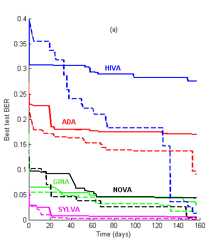
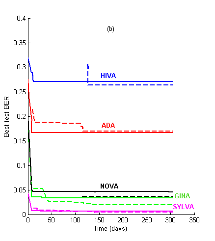 Figure 1: Learning curves. We show the evolution of the best test BER as a function of time for the 2006 and the 2007 challenges, using the same datasets. (a) Performance prediction challenge. Solid lines = test set BER. Dashed lines = validation set BER (note: validation set labels were released one month before the challenge ended). (b) AL vs. PK challenge. Solid lines = AL track. Dashed lines = PK track.
For the first few weeks of the challenge, the agnostic track (AL) results kept leading (see Figure 1). The learning curves all crossed at a certain point, except for ADA. After approximately 150 days the PK performance asymptote was reached. The asymptotic performances are reported at the top of Table 2. In contrast, last year, using the same data as the AL track, the competitors attained almost their best performances in about 60 days and kept slightly improving afterwards.
In Figure 1, we show the test BER distribution for all entries. There were about 60% more submissions in the AL track than in the PK track. This indicates that the “prior knowledge” track was harder to enter. However, the participants who did enter the PK track performed significantly better on average than those who entered the AL track, on all datasets except for HIVA. To quantify this observation we ran a Wilcoxon rank sum test on the difference between the median values of the two tracks (Table 2). We also performed paired comparisons for entrants who entered both tracks, using their last 5 submissions. In Table 2, a “+” indicates that the entrant performed best in the
PK track and a “-” indicates the opposite. We see that the entrants who entered both tracks did not always succeed in getting better results in the PK track. The pvalues of the sign test does not reveal any significant dominance of PK over AL or vice versa in that respect (all are between 0.25 and 0.5). However, for HIVA and NOVA the participants who entered both tracks failed to get better results in the PK track. We conclude that, while on average PK seems to win over AL, success is uneven and depends both on the domain and on the individuals’ expertise.
Table 2: Result statistics. The first 4 lines are computed from the test set BER over all entries, including reference entries made by the organizers. The indicate that PK wins over AL in most cases. The fifth line indicates that the median values of the 2 previous lines are significantly different (better for PK), except for HIVA. In the remainder of the table, a + indicates that in the 5 last entries of each participant having entered both tracks the best prior knowledge entry gets better results than the best agnostic entry. PK is better than AL for most entrants having entered both tracks for ADA, GINA and SYLVA, but the opposite is true for HIVA and NOVA (requiring more domain knwoledge). The last lign tests the significance of the fraction of times PK is better than AL or vice versa (no significance found because too few participants entered both tracks).
| ADA |
GINA | HIVA |
NOVA |
SYLVA | |
| Min PK BER | 0.170 | 0.019 | 0.264 | 0.037 | 0.004 |
| Min AL BER | 0.166 | 0.033 | 0.271 | 0.046 | 0.006 |
| Median PK BER | 0.189 | 0.025 | 0.31 | 0.047 | 0.008 |
| Median AL BER | 0.195 | 0.066 | 0.306 | 0.081 | 0.015 |
| Pval ranksum test | 5 E-08 | 3 E-18 | 0.25 | 8 E-08 | 1 E-18 |
| Jorge Sueiras | – | ||||
| Juha Reunanen | + | + | |||
| Marc Boulle | + | + | – | – | |
| Roman Lutz | + | ||||
| Vladimir Nikulin | – | + | + | ||
| Vojtech Franc | + | + | |||
| CWW | – | – | |||
| Reference (gcc) | + | + | – | ||
| Pvalue sign test | 0.31 | 0.19 | 0.25 | 0.25 | 0.3 |
BER distribution
In Figure 2, we show the test BER distribution for all entries. There were about 60% more submissions in the AL track than in the PK track. This indicates that the “prior knowledge” track was harder to enter. However, the participants who did enter the PK track performed significantly better on average than those who entered the AL track, on all datasets except for HIVA.
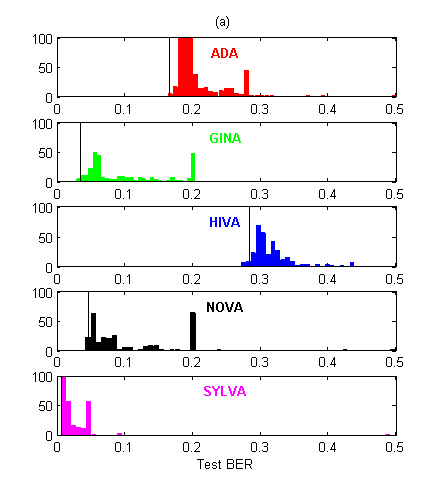
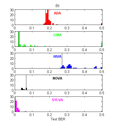
Figure 2: Histograms of BER performances. The thin vertical black line indicates the best entry counting toward the final ranking (among the five last of every entrant). (a) Agnostic learning track. (b) Prior knowledge track. Note that for NOVA, the best entries are not among the last ones submitted!
To quantify this observation we ran a Wilcoxon rank sum test on the difference between the median values of the two tracks (Table 2). We also performed paired comparisons for entrants who entered both tracks, using their last 5 submissions. In Table 2, a “+” indicates that the entrant performed best in the PK track and a “-” indicates the opposite. We see that the entrants who entered both tracks did not always succeed in getting better results in the PK track. The pvalues of the sign test does not reveal any significant dominance of PK over AL or vice versa in that respect (all are between 0.25 and 0.5). However, for HIVA and NOVA the participants who entered both tracks failed to get better results in the PK track. We conclude that, while on average PK seems to win over AL, success is uneven and depends both on the domain and on the individuals’ expertise.
Result tables
Here are the final result tables as of August 1st, 2007, which determined the prizes.
| Entrant | ADA | GINA | HIVA | NOVA | SYLVA | Score | Ave. best |
| Roman Lutz | 1 | 1 | 9 | 2 | 1 | 0.143101 | LogitBoost with trees |
| IDEAL, Intel | 2 | 2 | 4 | 9 | 6 | 0.237334 | out1-fs-nored-val |
| Juha Reunanen | 7 | 4 | 3 | 4 | 7 | 0.242436 | cross-indexing-8 |
| Vladimir Nikulin | 3 | 6 | 5 | 3 | 4 | 0.243593 | vn5 |
| H. Jair Escalante | 6 | 9 | 2 | 7 | 2 | 0.246381 | PSMS_100_4all_NCV |
| Mehreen Saeed | 9 | 5 | 10 | 1 | 3 | 0.278554 | Submit D final |
| Erinija Pranckeviene | 10 | 7 | 6 | 12 | 10 | 0.435781 | liknon feature selection |
| Joerg Wichard | 8 | 10 | 8 | 15 | 8 | 0.481145 | Final |
| Namgil Lee | 11 | 11 | 7 | 11 | 5 | 0.508458 | mlp+commitee+mcic |
| Vojtech Franc | 13 | 8 | 1 | 13 | 11 | 0.538075 | RBF SVM |
| Marc Boullé | 4 | 13 | 11 | 5 | 9 | 0.611149 | Data Grid |
| Zhihang Chen | 15 | 3 | 16 | 10 | 12 | 0.64688 | agnostic-resu-1 |
| Stijn Vanderlooy | 18 | 14 | 17 | 17 | 15 | 0.944741 | micc-ikat |
| Entrant | ADA | GINA | HIVA | NOVA | SYLVA | Score | Ave. best |
| Vladimir Nikulin | 2 | 1 | agnos | agnos | 3 | 0.0960 | vn3 |
| Juha Reunanen | agnos | 3 | agnos | agnos | 2 | 0.1294 | cross-indexing-prior-1a |
| Roman Lutz | agnos | agnos | agnos | agnos | 1 | 0.1381 | Doubleboost |
| Marc Boullé | 1 | 4 | agnos | 2 | 5 | 0.3821 | Data Grid |
| Jorge Sueiras | 3 | 5 | agnos | 1 | 4 | 0.3983 | boost tree |
| Vojtech Franc | 4 | 2 | agnos | agnos | agnos | 0.4105 | RBF SVM |
| Chloé Azencott (Baldi lab UCI) | agnos | agnos | 1 | agnos | agnos | 0.7640 | SVM |
The prize winners are indicated in yellow. The best average BER is held by Reference (Gavin Cawley): try to outperform him by making post-challenge entries! Louis Duclos-Gosselin is second on ADA with Neural Network13, and S. Joshua Swamidass (Baldi Lab, UCI) second on HIVA, but they are not entered in the table because they did not submit complete entries. The overall entry ranking is performed with the overall score (average rank over all datasets, using the test BER for ranking). The best performing complete entry may not contain all the best performing entries on the individual datasets.
From the results, we noticed that it is possible to do very well without prior knowledge and using prior knowledge skillfully is not that obvious:
- Datasets on which PK does not seem to buy a lot: On ADA and NOVA, the best results obtained by the participants is in the agnostic track! But it is possible to do better with prior knowledge: on ADA, the PK winner did worse in the AL track; the PK best “reference” entry yields best results on NOVA.
- Datasets on which PK is easy to exploit: On GINA and SYLVA, significantly better results are achieved in the PK track and all but one participant who entered both tracks did better with PK. However, the kind of prior knowledge used required little domain expertise.
- Dataset on which PK is hard to exploit: On HIVA, experts achieve significantly better results with prior knowledge, but non-experts entering both tracks do worse in the PK track. Here domain knowledge seems to play a key role.
The most successful classification methods in this competition involve boosting algorithms or kernel-based algorithms, such as support vector machines, with the exception of the data grid models, performing well on ADA. Approaches based on the provided CLOP package are among the top ranking entries. Model selection had to be harnessed to win the contest. The challenge results indicate that conducting an effective search is critical and that simple cross-validation (CV) can be used to effectively evaluate models.
We performed intermediate rankings using the test set (but not revealing the test set performances), see Table 5:
– December 1st, 2006 (for NIPS 06): Results of the model selection game. [Slides].
– March 1st , 2007: Competition deadline ranking. [Slides]
The March 1st results prompted us to extend the competition deadline because the participants in the “prior knowledge track” are still making progress, as indicated by the learning curves. The best results did not significantly improve, but some entrants made significant improvements in their methods.
| Dataset | IJCNN06A | NIPS06 A | March07A | March07P | IJCNN07A | IJCNN07P | Best result | Error bar |
| ADA | 0.1723 | 0.1660 | 0.1660 | 0.1756 | 0.1660 | 0.1756 | 0.1660 (agnos) | 0.0021 |
| GINA | 0.0288 | 0.0353 | 0.0339 | 0.0225 | 0.0339 | 0.0226 | 0.0192 (prior, ref) | 0.0009 |
| HIVA | 0.2757 | 0.2708 | 0.2827 | 0.2741 | 0.2827 | 0.2693 | 0.2636 (prior, ref) | 0.0068 |
| NOVA | 0.0445 | 0.0465 | 0.0463 | 0.0659 | 0.0456 | 0.0659 | 0.0367 (prior, ref) | 0.0018 |
| SYLVA | 0.0661 | 0.0065 | 0.0062 | 0.0043 | 0.0062 | 0.0043 | 0.0043 (prior) | 0.0004 |
Winning agnostic learning methods
The winner of the “agnostic learning” track is Roman Lutz, who also won the Performance Prediction Challenge (IJCNN06), using boosting techniques. Gavin Cawley, who joined the organization team and was co-winner of the previous challenge, made a reference entry using a kernel method called LSSVMs, which slightly outperforms that of Lutz. The improvements he made can partly be attributed to the introduction of an ARD kernel, which automatically downweighs the least relevant features and to a Bayesian regularization at the second level of inference. The second best entrant is the Intel group, also using boosting methods. The next best ranking entrants include Juha Reunanen and Hugo Jair Escalante, who have both been using CLOP models provided by the organizers and have proposed innovative search strategies for model selection: Escalante is using a biologically inspired particle swarm technique and Reunanen a cross-indexing method to make cross-validation more computationally efficient. Other top ranking participants in the AL track include Vladimir Nikulin and Joerg Wichard who both experimented with several ensemble methods, Erinija Pranckeviciene who performed a study of linear programming SVM methods (another kernel method), and Marc Boullé who introduced a new data grid method.
How to use prior knowledge?
We summarize the strategies employed by the participants to exploit prior knowledge on the various datasets.
ADA: the marketing application
The task of ADA is to discover high revenue people from census data, presented in the form of a two-class classification problem. The raw data from the census bureau is known as the Adult database in the UCI machine-learning repository. The 14 original attributes (features) represent age, workclass, education, education, marital status, occupation, native country, etc. and include continuous, binary and categorical features. The PK track had access to the original features and their descriptions. The AL track had access to a preprocessed numeric representation of the features, with a simple disjunctive coding of categorical variables, but the identity of the features was not revealed. We expected that the participants of the AL vs. PK challenge could gain in performance by optimizing the coding of the input features. Strategies adopted by the participants included using a thermometer code for ordinal variables (Gavin Cawley) and optimally grouping values for categorical variables (Marc Boullé). Boullé also optimally discretized continuous variables, which make them suitable for a naïve Bayes classifier. However, the advantage of using prior knowledge for ADA was marginal. The overall winner on ADA is in the agnostic track (Roman Lutz), and the entrants who entered both tracks and performed better using prior knowledge do not have results statistically significantly better. We conclude that optimally coding the variables may be not so crucial and that good performance can be obtained with a simple coding and a state-of-the-art classifier.
GINA: the handwriting recognition application
The task of GINA is handwritten digit recognition, the raw data is known as the MNIST dataset. For the “agnostic learning” track we chose the problem of separating two-digit odd numbers from two-digit even numbers. Only the unit digit is informative for this task, therefore at least 1/2 of the features are distractors. Additionally, the pixels that are almost always blank were removed and the pixel order was randomized to hide the meaning of the features. For the “prior knowledge” track, only the informative digit was provided in the original pixel map representation. In the PK track the identities of the digits (0 to 9) were provided for training, in addition to the binary target values (odd vs. even number). Since the prior knowledge track data consists of pixel maps, we expected the participants to perform image pre-processing steps such as noise filtering, smoothing, de-skewing, and feature extraction (points, loops, corners) and/or use kernels or architectures exploiting geometric invariance by small translation, rotation, and other affine transformations, which have proved to work well on this dataset. Yet, the participants to the PK track adopted very simple strategies, not involving a lot of domain knowledge. Some just relied on the performance boost obtained by the removal of the distractor features (Vladimir Nikulin, Marc Boullé, Juha Reunanen). Others exploited the knowledge of the individual class labels and created multi-class of hierarchical classifiers (Vojtech Franc, Gavin Cawley). Only the reference entries of Gavin Cawley (which obtained the best BER of 0.0192) included domain knowledge by using an RBF kernels with tunable receptive fields to smooth the pixel maps. In the future, it would be interesting to assess the methods of Simard et al on this data to see whether further improvements are obtained by exploiting geometrical invariances. The agnostic track data was significantly harder to analyze because of the hidden class heterogeneity and the presence of feature distractors. The best GINA final entry was therefore on the PK track and all four ranked entrants who entered both tracks obtained better results in the PK track. Further, the differences in performance are all statistically significant.
HIVA: the drug discovery application
The task of HIVA is to predict which compounds are active against the AIDS HIV infection. The original data from the NCI has 3 classes (active, moderately active, and inactive). We brought it back to a two-class classification problem (active & moderately active vs. inactive), but we provided the original labels for the “prior knowledge” track. The compounds are represented by their 3d molecular structure for the “prior knowledge” track (in SD format). For the “agnostic track” we represented the input data as vector of 2000 sparse binary variables. The variables represent properties of the molecule inferred from its structure by the ChemTK software package (version 4.1.1, Sage Informatics LLC). The problem is therefore to relate structure to activity (a QSAR – quantitative structure-activity relationship problem) to screen new compounds before actually testing them (a HTS – high-throughput screening problem). Note that in such applications the BER is not the best metric to assess performances since the real goal is to identify correctly the compounds most likely to be effective (belonging to the positive class). We resorted to using the BER to make comparisons easier across datasets. The raw data was not supplied in a convenient feature representation, which made it impossible to enter the PK track using agnostic learning methods, using off-the-shelf machine learning packages. The winner in HIVA (Chloé-Agathe Azencott of the Pierre Baldi Laboratory at UCI) is a specialist in this kind of dataset, on which she is working towards her PhD. She devised her own set of low level features, yielding a “molecular fingerprint” representation, which outperformed the ChemTK features used on the agnostic track. Her winning entry has a test BER of 0.2693, which is significantly better than the test BER of the best ranked AL entry of 0.2827 (error bar 0.0068). The results on HIVA are quite interesting because most agnostic learning entrants did not even attempt to enter the prior knowledge track and the entrants that did submit models for both tracks failed to obtain better results in the PK track. One of them working in an institute of pharmacology reported that too much domain knowledge is sometimes detrimental; experts in his institute advised against using molecular fingerprints, which ended up as the winning technique.
NOVA: the text classification application
The data of NOVA come from the 20-Newsgroup dataset. Each text to classify represents a message that was posted to one or several USENET newsgroups. The raw data is provided in the form of text files for the “prior knowledge” track. The preprocessed data for the “agnostic learning” track is a sparse binary representation using a bag-of-words with a vocabulary of approximately 17000 words (the features are simply frequencies of words in text). The original task is a 20-class classification problem but we grouped the classes into two categories (politics and religion vs. others) to make it a two-class problem. The original class labels were available for training in the PK track but not in the AL track. As the raw data consist of texts of variable length it was not possible to enter the PK track for NOVA without performing a significant pre-processing. All PK entrants in the NOVA track used a bag-ofwords representation, similar to the one provided in the agnostic track. Standard tricks were used, including stemming. Gavin Cawley used the additional idea of correcting the emails with an automated spell checker and Jorge Sueiras used a Thesaurus. No entrant who entered both tracks outperformed their AL entry with their PK entry in their last ranked entries, including the winner! This is interesting because the best PK entries made throughout the challenge significantly outperform the best AL entries (BER difference of 0.0089 for an error bar of 0.0018), see also Figure 1. Hence in this case, the PK entrants overfitted and were unable to select among their PK entries those, which would perform best on test data. This is not so surprising because the validation set on NOVA is quite small (175 examples). Even though the bag-of-words representation is known to be state-of-the-art for this kind of applications, it would be interesting to compare it with more sophisticated representations. To our knowledge, the best results on the 20 Newsgroup data were obtained by the method of distributional clustering by Ron Bekkerman.
SYLVA: the ecology application
The task of SYLVA is to classify forest cover types. The forest cover type for 30 x 30 meter cells was obtained from US Forest Service (USFS) Region 2 Resource Information System (RIS) data. We converted this into a two-class classification problem (classifying Ponderosa pine vs. everything else). The input vector for the “agnostic learning“ track consists of 216 input variables. Each pattern is composed of 4 records: 2 true records matching the target and 2 records picked at random. Thus 1/2 of the features are distractors. The “prior knowledge” track data is identical to the “agnostic learning” track data, except that the distractors are removed and the meaning of the features is revealed. For that track, the identifiers in the original forest cover dataset are revealed for the training set. As the raw data was already in a feature vector representation, this task was essentially testing the ability of the participants in the AL track to perform well in the presence of distractor features. The PK track winner (Roman Lutz) in his Doubleboost algorithm exploited the fact that each pattern was made of two records of the same pattern to train a classifier with twice as many training examples. Specifically, a new dataset was constructed by putting the second half of the data (variables 55 to 108) below the first half (variables 1 to 54). The new dataset is of dimension 2n times 54 (instead of n times 108). This new dataset is used for fitting the base learner (tree) of his boosting algorithm. The output of the base learner is averaged over the two records belonging to the same pattern. This strategy can be related to the neural network architectures using “shared weights”, whereby at training time, the weights trained on parts of the pattern having similar properties are constrained to be identical. This reduced the number of free parameters of the classifier.
Conclusions
For the first few month of the challenge, AL lead over PK, showing that the development of good AL classifiers is considerably faster. As of March 1st 2007, PK was leading over AL on four out of five datasets. We extended the challenge five more month, but the best performances did not significant improve during that time period. On datasets not requiring real expert domain knowledge (ADA, GINA, SYLVA), the participants entering both track obtained better results in the PK track, using a special-purpose coding of the inputs and/or the outputs, exploiting the knowledge of which features were uninformative, and using “shared weights” for redundantfeatures. For two datasets (HIVA and NOVA) the raw data was not in a feature representation and required some domain knowledge to preprocess data. The winning data representations consist in low level features (“molecular fingerprints” and “bag of words”). From the analysis of this challenge, we conclude that agnostic learning methods are very powerful. They quickly yield (in 40 to 60 days) to performances, which are near the best achievable performances. General-purpose techniques for exploiting prior knowledge in the encoding of inputs or outputs or the design of the learning machine architecture (e.g. via shared weights) may provide an additional performance boost, but exploiting real domain knowledge is both hard and time consuming. The net result of using domain knowledge rather using than low level features and relying on agnostic learning may actually be to worsen results, as experienced by some entrants. This fact seems to be a recurrent theme in machine learning publications and the results of our challenge confirm it. Future work includes incorporating the best identified methods in our challenge toolkit CLOP. The challenge web site remains open for post-challenge submissions.